Python 教程中的 SciPy：什么是 |库和函数示例

Python 中的 SciPy
Python 中的 SciPy 是一个开源库，用于解决数学、科学、工程和技术问题。它允许用户使用各种高级 Python 命令来操作数据和可视化数据。 SciPy 建立在 Python NumPy 扩展之上。 SciPy 也发音为“Sigh Pi”。

SciPy 的子包：

文件输入/输出 - scipy.io

特殊功能 - scipy.special

线性代数运算 - scipy.linalg

插值 - scipy.interpolate

优化和适配 - scipy.optimize

统计和随机数 - scipy.stats

数值积分 - scipy.integrate

快速傅里叶变换 - scipy.fftpack

信号处理 - scipy.signal

图像处理 - scipy.ndimage

在本 Python SciPy 教程中，您将学习：

什么是 SciPy？

为什么使用 SciPy

Numpy VS SciPy

SciPy – 安装和环境设置

文件输入/输出包：

特殊功能包：

使用 SciPy 进行线性代数：

离散傅里叶变换 - scipy.fftpack

SciPy 中的优化和拟合 - scipy.optimize

Nelder –Mead 算法：

使用 SciPy 进行图像处理 – scipy.ndimage

为什么使用 SciPy

SciPy 包含各种子包，有助于解决与科学计算相关的最常见问题。

Python 中的 SciPy 包是使用最多的科学库，仅次于 GNU Scientific Library for C/C++ 或 Matlab。

易于使用和理解以及快速的计算能力。

它可以对 NumPy 库数组进行操作。

Numpy VS SciPy

麻木：

Numpy 是用 C 语言编写的，用于数学或数值计算。
它比其他 Python 库更快
Numpy 是数据科学执行基本计算的最有用的库。
Numpy 只包含数组数据类型，它执行最基本的操作，如排序、整形、索引等。

科学：

SciPy 构建在 NumPy 之上
Python 中的 SciPy 模块是线性代数的全功能版本，而 Numpy 仅包含一些功能。
大多数新的数据科学功能都在 Scipy 而不是 Numpy 中可用。

SciPy – 安装和环境设置

你也可以通过 pip 在 Windows 中安装 SciPy

Python3 -m pip install --user numpy scipy

在 Linux 上安装 Scipy

sudo apt-get install  python-scipy python-numpy

在 Mac 上安装 SciPy

sudo port install py35-scipy py35-numpy

在我们开始学习 SciPy Python 之前，您需要了解 NumPy 数组的基本功能以及不同类型的数组

导入 SciPy 模块和 Numpy 的标准方法：

from scipy import special   #same for other modules
import numpy as np

文件输入/输出包：

Scipy，I/O 包，具有广泛的功能，可处理不同的文件格式，包括 Matlab、Arff、Wave、Matrix Market、IDL、NetCDF、TXT、CSV 和二进制格式。

让我们以 MatLab 中常用的一种文件格式 Python SciPy 为例：

 import numpy as np
 from scipy import io as sio
 array = np.ones((4, 4))
 sio.savemat('example.mat', {'ar': array}) 
 data = sio.loadmat(‘example.mat', struct_as_record=True)
 data['ar']

输出：

array([[ 1., 1., 1., 1.],
           [ 1., 1., 1., 1.],
           [ 1., 1., 1., 1.],
           [ 1., 1., 1., 1.]])

代码说明

第 1 行和第 2 行： 使用 I/O 包和 Numpy 在 Python 中导入基本的 SciPy 库。
第 3 行 :创建 4 x 4 维数组
第 4 行 :在 example.mat 中存储数组文件。
第 5 行： 从 example.mat 获取数据文件
第 6 行 ：打印输出。

特殊功能包

scipy.special 软件包包含许多数学物理函数。
SciPy 特殊函数包括立方根、指数、对数和指数、Lambert、Permutation and Combinations、Gamma、Bessel、超几何、Kelvin、beta、抛物柱面、相对误差指数等。
对于所有这些功能的一行描述，请在 Python 控制台中输入：

help(scipy.special)	
Output : 
NAME
    scipy.special

DESCRIPTION
    ========================================
    Special functions (:mod:`scipy.special`)
    ========================================
     
    .. module:: scipy.special
     
    Nearly all of the functions below are universal functions and follow
    broadcasting and automatic array-looping rules. Exceptions are noted.

三次方根函数：

Cubic Root 函数求值的立方根。

语法：

scipy.special.cbrt(x)

示例：

from scipy.special import cbrt
#Find cubic root of 27 & 64 using cbrt() function
cb = cbrt([27, 64])
#print value of cb
print(cb)

输出： 数组([3., 4.])

指数函数：

指数函数按元素计算 10**x。

示例：

from scipy.special import exp10
#define exp10 function and pass value in its
exp = exp10([1,10])
print(exp)

输出：[1.e+01 1.e+10]

排列与组合：

SciPy 还提供了计算排列和组合的功能。

组合—— scipy.special.comb(N,k)

示例：

from scipy.special import comb
#find combinations of 5, 2 values using comb(N, k)
com = comb(5, 2, exact = False, repetition=True)
print(com)

输出：15.0

排列——

scipy.special.perm(N,k)

示例：

from scipy.special import perm
#find permutation of 5, 2 using perm (N, k) function
per = perm(5, 2, exact = True)
print(per)

输出：20

对数和指数函数

Log Sum Exponential 计算总和指数输入元素的对数。

语法：

scipy.special.logsumexp(x)

贝塞尔函数

N次整数阶计算函数

语法：

scipy.special.jn()

SciPy 线性代数

SciPy 的线性代数是 BLAS 和 ATLAS LAPACK 库的实现。
与 BLAS 和 LAPACK 相比，线性代数的性能非常快。
线性代数例程接受二维数组对象，输出也是二维数组。

现在让我们用 scipy.linalg, 做一些测试

计算行列式 一个二维矩阵，

from scipy import linalg
import numpy as np
#define square matrix
two_d_array = np.array([ [4,5], [3,2] ])
#pass values to det() function
linalg.det( two_d_array )

输出： -7.0

逆矩阵——

scipy.linalg.inv()

Scipy的逆矩阵计算任何方阵的逆。

来看看吧，

from scipy import linalg
import numpy as np
# define square matrix
two_d_array = np.array([ [4,5], [3,2] ])
#pass value to function inv()
linalg.inv( two_d_array )

输出：

array( [[-0.28571429,  0.71428571],
       [ 0.42857143, -0.57142857]] )

特征值和特征向量

scipy.linalg.eig()

线性代数中最常见的问题是特征值和特征向量，可以使用eig()轻松解决功能。
现在让我们找到 (X 的特征值 ) 和对应的二维方阵特征向量。

示例

from scipy import linalg
import numpy as np
#define two dimensional array
arr = np.array([[5,4],[6,3]])
#pass value into function
eg_val, eg_vect = linalg.eig(arr)
#get eigenvalues
print(eg_val)
#get eigenvectors
print(eg_vect)

输出：

[ 9.+0.j -1.+0.j] #eigenvalues
 [ [ 0.70710678 -0.5547002 ] #eigenvectors
   [ 0.70710678  0.83205029] ]

离散傅里叶变换 - scipy.fftpack

DFT 是一种数学技术，用于将空间数据转换为频率数据。
FFT（Fast Fourier Transformation）是一种计算DFT的算法
FFT 应用于多维数组。
频率定义了特定时间段内信号或波长的数量。

示例： 使用 Matplotlib 库来一波展示。我们以 sin(20 × 2πt) 的简单周期函数为例

%matplotlib inline
from matplotlib import pyplot as plt
import numpy as np 

#Frequency in terms of Hertz
fre  = 5 
#Sample rate
fre_samp = 50
t = np.linspace(0, 2, 2 * fre_samp, endpoint = False )
a = np.sin(fre  * 2 * np.pi * t)
figure, axis = plt.subplots()
axis.plot(t, a)
axis.set_xlabel ('Time (s)')
axis.set_ylabel ('Signal amplitude')
plt.show()

输出：

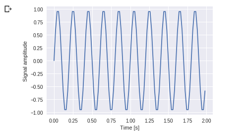
你可以看到这个。频率为 5 Hz，其信号在 1/5 秒内重复 - 它被称为特定时间段。

现在让我们在 DFT 应用程序的帮助下使用这个正弦波。

from scipy import fftpack

A = fftpack.fft(a)
frequency = fftpack.fftfreq(len(a)) * fre_samp
figure, axis = plt.subplots()

axis.stem(frequency, np.abs(A))
axis.set_xlabel('Frequency in Hz')
axis.set_ylabel('Frequency Spectrum Magnitude')
axis.set_xlim(-fre_samp / 2, fre_samp/ 2)
axis.set_ylim(-5, 110)
plt.show()

输出：

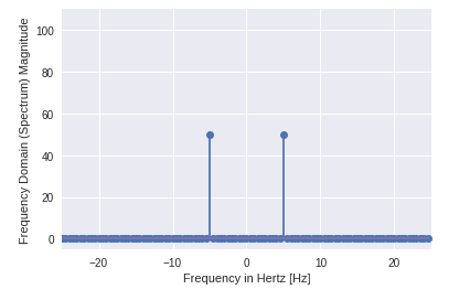
可以清楚的看到输出是一个一维数组。
包含复数的输入除两个点外为零。
在 DFT 示例中，我们将信号的幅度可视化。

SciPy 中的优化和拟合 - scipy.optimize

优化为最小化曲线拟合、多维或标量和根拟合提供了一种有用的算法。
我们举一个标量函数的例子， 找到最小标量函数.

%matplotlib inline
import matplotlib.pyplot as plt
from scipy import optimize
import numpy as np

def function(a):
       return   a*2 + 20 * np.sin(a)
plt.plot(a, function(a))
plt.show()
#use BFGS algorithm for optimization
optimize.fmin_bfgs(function, 0)

输出：

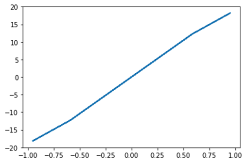
优化成功终止。

当前函数值：-23.241676

迭代次数：4

功能评价：18

梯度评价：6

数组([-1.67096375])

在这个例子中，优化是在梯度下降算法的帮助下从初始点开始的
但可能的问题是局部最小值而不是全局最小值。如果我们没有找到全局最小值的邻居，那么我们需要应用全局优化并找到用作 basinhopping() 的全局最小值函数它结合了本地优化器。

optimize.basinhopping(function, 0)

输出：

fun: -23.241676238045315
 lowest_optimization_result:
      fun: -23.241676238045315
 hess_inv: array([[0.05023331]])
      jac: array([4.76837158e-07])
  message: 'Optimization terminated successfully.'
     nfev: 15
      nit: 3
     njev: 5
   status: 0
  success: True
        x: array([-1.67096375])
                    message: ['requested number of basinhopping iterations completed successfully']
      minimization_failures: 0
                       nfev: 1530
                        nit: 100
                       njev: 510
               x: array([-1.67096375])

Nelder – 米德算法：

Nelder-Mead 算法通过方法参数进行选择。
它为公平行为函数提供了最直接的最小化方法。
Nelder – Mead 算法不用于梯度评估，因为它可能需要更长的时间才能找到解决方案。

import numpy as np
from scipy.optimize import minimize
#define function f(x)
def f(x):   
    return .4*(1 - x[0])**2
  
optimize.minimize(f, [2, -1], method="Nelder-Mead")

输出：

final_simplex: (array([[ 1.        , -1.27109375],
       [ 1.        , -1.27118835],
       [ 1.        , -1.27113762]]), array([0., 0., 0.]))
           fun: 0.0
       message: 'Optimization terminated successfully.'
          nfev: 147
           nit: 69
        status: 0
       success: True
             x: array([ 1.        , -1.27109375])

使用 SciPy 进行图像处理 – scipy.ndimage

scipy.ndimage 是 SciPy 的一个子模块，主要用于执行图像相关操作
ndimage 表示“n”维图像。
SciPy 图像处理提供几何变换（旋转、裁剪、翻转）、图像过滤（锐化和去噪）、显示图像、图像分割、分类和特征提取。
MISC 包 在 SciPy 中包含可用于执行图像处理任务的预构建图像

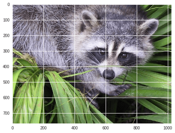
示例： 我们以图像的几何变换为例

from scipy import misc
from matplotlib import pyplot as plt
import numpy as np
#get face image of panda from misc package
panda = misc.face()
#plot or show image of face
plt.imshow( panda )
plt.show()

输出：

现在我们向下翻转 当前图片：

#Flip Down using scipy misc.face image  
flip_down = np.flipud(misc.face())
plt.imshow(flip_down)
plt.show()

输出：

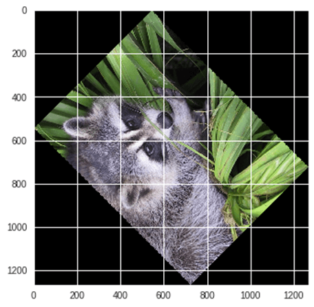
示例： 使用 Scipy 旋转图像，

from scipy import ndimage, misc
from matplotlib import pyplot as plt
panda = misc.face()
#rotatation function of scipy for image – image rotated 135 degree
panda_rotate = ndimage.rotate(panda, 135)
plt.imshow(panda_rotate)
plt.show()

输出：

与 Scipy 集成 - 数值积分

当我们对任何无法解析积分的函数进行积分时，我们需要转向数值积分
SciPy 提供了将函数与数值积分相结合的功能。
scipy.integrate 库有单积分、双积分、三重积分、多积分、高斯平方、Romberg、梯形和辛普森规则。

示例： 现在举一个单一集成的例子

这里a 是上限，b 是下限

from scipy import integrate
# take f(x) function as f
f = lambda x : x**2
#single integration with a = 0 & b = 1  
integration = integrate.quad(f, 0 , 1)
print(integration)

输出：

(0.33333333333333337, 3.700743415417189e-15)

这里函数返回两个值，其中第一个值是积分，第二个值是积分估计误差。

示例：现在以 双重积分的 SciPy 示例为例。 我们找到以下方程的二重积分，

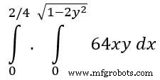
from scipy import integrate
import numpy as np
#import square root function from math lib
from math import sqrt
# set  fuction f(x)
f = lambda x, y : 64 *x*y
# lower limit of second integral
p = lambda x : 0
# upper limit of first integral
q = lambda y : sqrt(1 - 2*y**2)
# perform double integration
integration = integrate.dblquad(f , 0 , 2/4,  p, q)
print(integration)

输出：

(3.0, 9.657432734515774e-14)

您已经看到上面的输出与之前的输出相同。

总结

SciPy（发音为“Sigh Pi”）是一个基于 Python 的开源库，用于数学、科学计算、工程和技术计算。
SciPy 包含各种子包，有助于解决与科学计算相关的最常见问题。
SciPy 构建在 NumPy 之上

包名	说明
scipy.io	文件输入/输出
scipy.special	特殊功能
scipy.linalg	线性代数运算
scipy.interpolate	插值
scipy.optimize	优化与适配
scipy.stats	统计数据和随机数
scipy.integrate	数值积分
scipy.fftpack	快速傅里叶变换
scipy.signal	信号处理
scipy.ndimage	图像处理 –

Python readline() 方法和示例如何在 Python 中读取 CSV 文件CSV文件读写

Python