工厂工程师的可靠性工程原则

负责制造和其他工业活动的经理和工程师越来越多地将可靠性重点纳入他们的战略和战术计划和举措中。这一趋势正在影响许多职能领域，包括机器/系统设计和采购、工厂运营和工厂维护。

可靠性工程起源于航空业，作为一门学科，历来主要侧重于确保产品可靠性。这些方法越来越多地被用来确保制造工厂和设备的生产可靠性——通常作为精益制造的推动者。本文介绍了这些用于工厂可靠性工程的方法中最相关和最实用的方法，包括：

• 故障率、MTBF、可用性等的基本可靠性计算。
• 指数分布简介——可靠性方法的基石。
• 使用多功能 Weibull 系统识别故障时间依赖性。
• 开发有效的现场数据收集系统。

可靠性工程历史

可靠性工程领域的起源，至少是对它的需求，可以追溯到人类开始依赖机器谋生的那一刻。例如，Noria 是一种古老的泵，被认为是世界上第一台精密机器。诺里亚人利用河流或溪流中的水力能，利用水桶将水输送到水槽、高架桥和其他分配装置，以灌溉田地并为社区供水。

如果社区 Noria 失败，依靠它来供应食物的人们将处于危险之中。生存一直是可靠性和可靠性的重要动力来源。

虽然其需求的起源是古老的，但作为一门技术学科的可靠性工程随着二战后商业航空的发展而真正蓬勃发展。航空业公司的经理们很快意识到坠机对企业不利。 Quality Progress 的编辑 Karen Bernowski 1994年，麻省理工学院统计学教授阿诺德·巴内特（Arnold Barnett）在她的一篇社论中揭示了通过各种方式对死亡的媒体价值进行的研究。

巴内特通过各种方式评估了每 1000 人死亡时纽约时报头版新闻文章的数量。他发现，与癌症相关的死亡每 1000 人中有 0.02 篇头版新闻文章，每 1000 人中有 1.7 篇是凶杀案，每 1000 人中有 2.3 篇是艾滋病，每 1000 人中有 2.3 篇与航空相关的事故！

航空相关事故的成本和引人注目的性质有助于激励航空业大力参与可靠性工程学科的发展。同样，由于国防军事装备的关键性质，长期以来一直采用可靠性工程技术来确保作战准备就绪。我们在可靠性工程领域的许多标准都是 MIL 标准或起源于军事活动。

什么是可靠性工程？

可靠性工程涉及零件、产品和系统的寿命和可靠性。更令人痛心的是，它是关于控制风险的。可靠性工程结合了多种分析技术，旨在帮助工程师了解这些部件、产品和系统的故障模式和模式。传统上，可靠性工程领域主要关注产品的可靠性和可靠性保证。

近年来，在生产环境中部署机器和其他物理资产的组织已经开始部署各种可靠性工程原则，以实现生产可靠性和可靠性保证。

生产组织越来越多地部署可靠性工程技术，例如以可靠性为中心的维护 (RCM)，包括故障模式和影响（和临界性）分析 (FMEA、FMECA)、根本原因分析 (RCA)、基于条件的维护、改进的工作计划方案、等。这些组织开始采用基于生命周期成本的设计和采购策略、变更管理方案和其他先进的工具和技术，以控制可靠性差的根本原因。

然而，生产可靠性保证社区采用可靠性工程的更多定量方面的速度很慢。这部分是由于技术的复杂性，部分是由于难以获得有用的数据。

从表面上看，可靠性工程的定量方面可能看起来复杂而艰巨。然而，实际上，对最基本和最广泛适用的方法的相对基本的了解可以使工厂可靠性工程师更清楚地了解问题发生的位置、问题的性质及其对生产过程的影响——至少在数量上感。

如果使用得当，定量可靠性工程工具和方法使工厂可靠性工程能够更有效地应用 RCM、RCA 等提供的框架，从而消除与其应用相关的一些猜测。但是，工程师在应用这些方法时必须特别聪明。

为什么？与产品可靠性保证的某种一维世界相比，生产过程的操作环境和环境包含更多的变量。这是由于设计工程、采购、生产/运营、维护等的综合影响，以及难以创建有效的测试和实验来模拟典型生产环境的多维方面。

尽管在生产环境中应用定量可靠性方法越来越困难，但对工具有充分的了解并在适当的时候应用它们是值得的。定量数据有助于定义问题/机会的性质和大小，从而为他或她应用其他可靠性工程工具的可靠性提供愿景。

本文将介绍适用于对生产可靠性保证感兴趣的工厂工程师的最基本的可靠性工程方法。它的前提是对代数、概率论和基于高斯（正态）分布的单变量统计有基本的了解（例如集中趋势的度量、离散和可变性的度量、置信区间等）。

需要说明的是，本文是对可靠性方法的简要介绍。它绝不是对可靠性工程方法的全面调查，也绝不是新的或非常规的。此处描述的方法是可靠性工程师经常使用的方法，是那些寻求美国质量协会 (ASQ) 可靠性工程师 (CRE) 专业认证的人员的核心知识概念。

本文的参考书目中列出了几本有关可靠性工程的书籍。这篇文章的作者找到了工程师的可靠性方法 由 K.S. Krishnamoorthi 和可靠性统计 Robert Dovich 撰写的关于可靠性工程方法主题的特别有用且用户友好的参考资料。两者均由 ASQ 出版社出版。

在讨论方法之前，您应该熟悉可靠性工程术语。为方便起见，本文附录中提供了关键术语和定义的高度删节列表。有关可靠性术语和命名法的更详尽定义，请参阅 MIL-STD-721 和其他相关标准。附录中的定义来自MIL-STD-721。

可靠性工程中的基本数学概念

许多数学概念适用于可靠性工程，尤其是概率和统计领域。同样，许多数学分布可用于各种目的，包括高斯（正态）分布、对数正态分布、瑞利分布、指数分布、威布尔分布等。

出于简要介绍的目的，我们将讨论仅限于指数分布和威布尔分布，这两种分布在可靠性工程中应用最为广泛。为简洁起见，已排除重要的数学概念，例如分布拟合优度和置信区间。

故障率和平均故障间隔时间（MTBF/MTTF）

定量可靠性测量的目的是定义相对于时间的故障率，并在数学分布中对该故障率进行建模，以了解故障的定量方面。最基本的构建块是故障率，它使用以下等式估算：

其中：
λ =失效率（有时称为危险率）
T =总运行时间/周期/英里/等。在失败和非失败项目的调查期间。
r =调查期间发生的故障总数。

例如，如果五台电动机总共运行 50 年，在此期间出现 5 次功能故障，则故障率为每年 0.1 次故障。

另一个非常基本的概念是平均故障间隔时间（MTBF/MTTF）。 MTBF 和 MTTF 之间的唯一区别是我们在提及故障时修复的项目时使用 MTBF。对于简单扔掉和更换的物品，我们使用术语 MTTF。计算方式相同。

估计平均故障间隔时间 (MTBF) 和平均故障时间 (MTTF) 的基本计算是集中趋势的两种度量，只是故障率函数的倒数。它是使用以下公式计算的。

其中：
θ =平均间隔时间/失败时间
T =总运行时间/周期/英里/等。在失败和非失败项目的调查期间。
r =调查期间发生的故障总数。

我们工业电机示例的 MTBF 是 10 年，这是电机故障率的倒数。顺便说一下，我们会估计故障时重建的电动机的 MTBF。对于被认为是一次性的小型电机，我们将集中趋势的度量表示为 MTTF。

失效率是许多更复杂的可靠性计算的基本组成部分。根据机械/电气设计、操作环境、环境和/或维护效率，机器的故障率随时间的变化可能会下降、保持不变、线性增加或几何增加（图 1）。稍后将更详细地讨论故障率与时间的重要性。

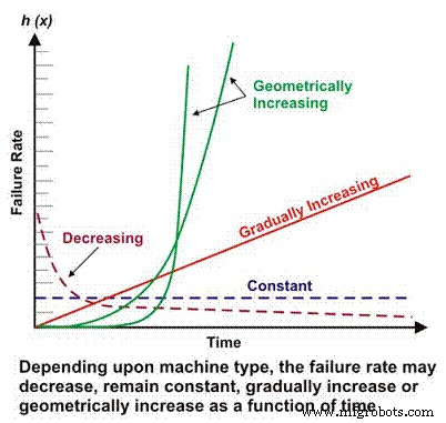
图 1. 不同故障率与时间情景

“浴缸”曲线

仅接受过概率和统计基础培训的个人可能最熟悉高斯分布或正态分布，后者与熟悉的钟形概率密度曲线相关。高斯分布通常适用于两个最常见的集中趋势度量（均值和中值）近似相等的数据集。

令人惊讶的是，尽管高斯分布在建模从标准化考试分数到婴儿出生体重等各种现象的概率方面具有多功能性，但它并不是可靠性工程中采用的主要分布。高斯分布在评估具有主导故障模式的机器的故障特征方面占有一席之地，但可靠性工程中采用的主要分布是指数分布。

在评估机器的可靠性和故障特性时，我们必须从备受诟病的“浴缸”曲线开始，它反映了故障率与时间的关系（图 2）。在概念上，浴盆曲线有效地展示了机器的三个基本故障率特征：下降、恒定或增加。遗憾的是，浴缸曲线在维修工程文献中受到严厉批评，因为它无法有效地模拟工厂中大多数机器的特征故障率，而这在宏观层面上是普遍存在的。

大多数机器在生命早期、婴儿死亡率和/或浴缸曲线的恒定故障率区域中度过一生。我们很少在工业机器中看到系统性基于时间的故障。尽管在对典型工业机器的故障率建模方面存在局限性，但浴盆曲线是解释可靠性工程基本概念的有用工具。

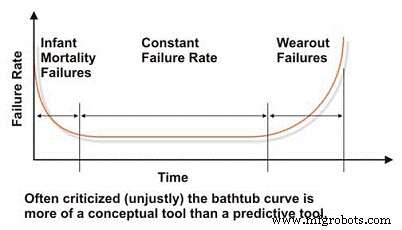
图 2. 备受诟病的“浴缸”曲线

人体是遵循浴缸曲线的系统的一个很好的例子。人和其他有机物种在生命的最初几年，尤其是最初几年，往往会遭受很高的失败率（死亡率），但随着孩子年龄的增长，失败率会降低。假设一个人进入青春期并在他或她的青少年时期幸存下来，他或她的死亡率会变得相当稳定并一直保持下去，直到年龄（时间）相关疾病开始增加死亡率（疲劳）。

许多影响因素会影响死亡率，包括产前护理和母亲的营养、医疗保健的质量和可用性、环境和营养、生活方式的选择，当然还有遗传倾向。这些因素可以比喻为影响机器寿命的因素。设计和采购类似于遗传倾向；安装和调试类似于产前护理和母亲的营养；生活方式的选择和医疗服务的可用性类似于维护有效性和对操作条件的主动控制。

指数分布

指数分布是最基本和最广泛使用的可靠性预测公式，它对具有恒定故障率的机器或浴盆曲线的平坦部分进行建模。大多数工业机器的大部分时间都在恒定的故障率中度过，因此它的适用范围很广。以下是用于估计遵循指数分布的机器可靠性的基本方程，其中故障率作为时间的函数是恒定的。

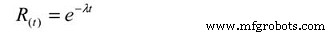
其中：
R(t) =一段时间、周期、英里等 (t) 的可靠性估计。
e =自然对数的底数 (2.718281828)
λ =故障率（1/MTBF，或 1/MTTF）

在我们的电动机示例中，如果假设故障率恒定，则电动机运行 6 年没有故障的可能性或预计可靠性为 55%。计算如下：
R(6) =2.718281828-(0.1* 6)
R(6) =0.5488 =~ 55%

换句话说，六年后，在相同应用中运行的相同电机中约有 45% 可能会出现故障。在这一点上值得重申的是，这些计算预测了人口的概率。群体中的任何特定个体都可能在操作的第一天失败，而另一个个体可能会持续 30 年。这就是概率可靠性预测的本质。

指数分布的一个特征是 MTBF 出现在计算出的可靠性为 36.78% 的点，或者 63.22% 的机器已经发生故障的点。在我们的电机示例中，在 10 年后，在相同应用中使用的相同电机群中的 63.22% 的电机预计会出现故障。也就是说，存活率为36.78%。

我们经常将预计轴承寿命称为 L10 寿命。这是预计 10% 的轴承群会出现故障（90% 的存活率）的时间点。实际上，只有一小部分轴承能够存活到 L10 点。当我们或许应该将目光投向 L63.22 点时，我们已经开始接受这是轴承的客观寿命，这表明我们的轴承平均可以持续到预计的 MTBF——当然，假设轴承服从指数分布。我们稍后将在本文的威布尔分析部分讨论该问题。

概率密度函数 (pdf) 或寿命分布是近似失效频率分布的数学方程。是 pdf 或寿命频率分布，在高斯分布或正态分布中产生熟悉的钟形曲线。以下是指数分布的pdf。

其中：
pdf(t) =给定时间 (t) 的寿命频率分布
e =自然对数的底数 (2.718281828)
λ =故障率（1/MTBF，或 1/MTTF）

在我们的电动机示例中，三年后实际发生故障的可能性计算如下：
pdf(3) =01. * 2.718281828-(0.1* 3)
pdf(3) =0.1 * 0.7408
pdf(3) =.07408 =~ 7.4%

在我们的例子中，如果我们假设一个恒定的故障率，它遵循指数分布，工业电动机的寿命分布或 pdf 表示在图 3 中。 不要被 pdf 函数的下降性质所迷惑。是的，故障率是恒定的，但 pdf 在数学上假设故障没有替换，因此可能发生故障的数量不断减少 - 渐近接近于零。

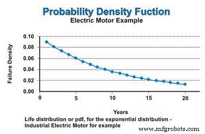
图 3. 概率密度函数 (pdf)

累积分布函数 (cdf) 只是人们在一段时间内可能预期的累积故障数。对于指数分布，故障率是恒定的，因此将故障组件添加到 cdf 的相对速率保持恒定。但是，由于故障导致总体数量下降，因此数学估计的实际故障数量会随着数量的减少而减少。就像 pdf 渐近逼近 0 一样，cdf 渐近逼近 1（图 4）。

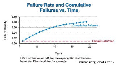
图 4. 故障率和累积分布函数

浴缸曲线的故障率下降部分（通常称为婴儿死亡率区域）和磨损区域将在下一节讨论多功能威布尔分布。

威布尔分布

Weibull 分析最初由瑞典数学家 Wallodi Weibull 开发，很容易成为可靠性工程师采用的最通用的分布。虽然它被称为分布，但它实际上是一种工具，它使可靠性工程师能够首先表征一组失效数据的概率密度函数（失效频率分布），以将失效表征为早期寿命、常数（指数）或磨损（高斯或对数正态分布）通过在特殊绘图纸上绘制失效时间数据，并用失效时间/周期/英里数的对数绘制对数缩放的 X 轴与日志上每个失效所代表的累积百分比-log 缩放 Y 轴（图 5）。

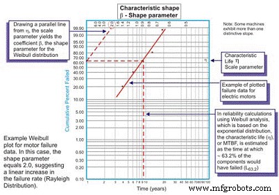
图 5. 简单的威布尔图 – 注释

绘制后，合成曲线的线性斜率是一个重要变量，称为形状参数，用 â 表示，用于调整指数分布以拟合大量失效分布。一般来说，如果 â 系数或形状参数小于 1.0，则该分布表现出早期生命或婴儿死亡失败。如果形状参数超过约 3.5，则数据具有时间依赖性，表明磨损失效。

该数据集通常采用高斯分布或正态分布。随着 â 系数增加到 ~ 3.5 以上，钟形分布收紧，显示出增加的峰度（曲线顶部的峰值）和更小的标准偏差。许多数据集会表现出两个甚至三个不同的区域。

例如，可靠性工程师通常绘制一条曲线表示磨合期间的形状参数，另一条曲线表示恒定或逐渐增加的故障率。在某些情况下，会出现第三种明显的线性斜率来识别第三种形状，即磨损区域。

在这些情况下，故障数据的 pdf 实际上确实采用了熟悉的浴盆曲线形状（图 6）。然而，工厂中使用的大多数机械设备都表现出婴儿死亡率区域和恒定或逐渐增加的故障率区域。很少能看到代表磨损的曲线出现。特征寿命或 η（小写希腊语“Eta”）是 MTBF 的威布尔近似值。 63.21% 的被评估单元失败总是时间、英里或周期的函数，这就是指数分布的 MTBF/MTTF。

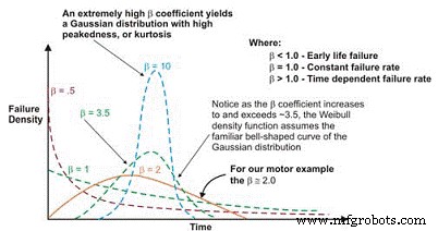
图 6. 根据形状参数，威布尔失效密度曲线可以假设多个分布，这就是它在可靠性工程中如此通用的原因。

作为将此工具与卓越维护和卓越运营联系起来的警告，如果我们要更有效地控制导致轴承、齿轮等机械故障的强制功能，例如润滑、污染控制、对齐、平衡、适当的操作等，更多的机器实际上会达到它们的疲劳寿命。达到疲劳寿命的机器会表现出熟悉的磨损特性。

使用 β 系数将失效率方程调整为时间的函数，得出以下通用方程：

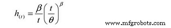
其中：
h(t) =给定时间 (t) 的失效率（或危险率）
e =自然对数的底 (2.718281828)
θ =估计的 MTBF/MTTF
β =图中的威布尔形状参数。

并且，以下可靠性函数：

其中：
R(t) =一段时间、周期、英里等的可靠性估计。(t)
e =自然对数的底 (2.718281828)
θ =估计的 MTBF/MTTF
β =图中的威布尔形状参数。

并且，以下概率密度函数（pdf）：

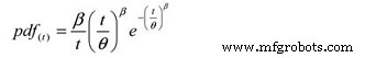
其中：
pdf(t) =一段时间内的概率密度函数估计，
周期、英里等 (t)
e =自然对数的底 (2.718281828)
θ =估计的 MTBF/MTTF
β =图中的威布尔形状参数。

需要说明的是，当 β 等于 1.0 时，威布尔分布呈指数分布形式，并以此为基础。

对于外行来说，执行威布尔分析所需的数学可能看起来令人生畏。但是一旦你理解了公式的原理，数学就非常简单了。此外，软件将为我们今天完成大部分工作，但重要的是要了解基础理论，以便工厂可靠性工程师能够有效地部署强大的威布尔分析技术。

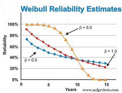
在我们之前讨论的电动机示例中，我们之前假设了指数分布。然而，如果威布尔分析通过产生 0.5 的 β 形状参数来揭示早期寿命故障，则六年时的可靠性估计将是~46%，而不是假设指数分布的~55%。为了减少磨损故障，我们需要依靠我们的供应商提供更好的制造和交付质量和可靠性，更好地存放电机以避免生锈、腐蚀、微动和其他静态磨损机制，并更好地完成安装并启动新的或重建的机器。

相反，如果威布尔分析显示电机主要表现出与磨损相关的故障，产生 5.0 的 β 形状参数，则六年时间的可靠性估计将是 ~ 93%，而不是假设指数分布的 ~55% 估计。对于与时间相关的磨损故障，我们可以执行计划检修或更换，假设我们在到达磨损区域后对 MTBF/MTTF 有一个很好的估计，并且标准偏差足够小，以便做出高可信度的重建/更换决策成本并不高。

在我们的电机示例中，假设 β 形状参数为 5.0，故障率在大约五六年后开始迅速增加，因此在估计基于时间的更换或重建时，我们可能希望编辑数据以仅关注磨损区域时间。或者，我们可以改进设计，针对主要失效模式，以减少“应力-强度”干扰。换句话说，我们可以尝试通过设计修改来消除机器的弱点，目标是消除任何导致时间相关故障的因素。

假设一切都是常数，除了 β 形状参数，图 7 说明了 β 形状参数对可靠性估计的差异，假设 β 形状值为 0.5（早期寿命）、1.0（常数或指数）和 5.0（磨损）一系列时间估计。此图直观地说明了风险随时间增加 (β =0.5)、风险随时间恒定 (β =1.0) 和风险随时间增加 (β =5) 的概念。

图 7. 作为时间函数的不同可靠性预测威布尔形状参数

多斜率威布尔图

通常，当通过威布尔图上的数据点绘制最佳拟合回归线时，相关系数很差，这意味着实际数据点与回归线的距离很远。这是通过检查相关系数 R 或更保守的 R2 来评估的，R2 表示数据可变性。当相关性较差时，可靠性工程师应检查数据以评估是否存在两种或多种模式，这可以表示故障模式、操作环境等方面的主要差异。通常，这会产生两个或更多的 beta 估计值（图 8）。

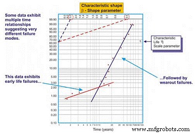
图 8. 多 beta 威布尔图示例

正如我们在图 8 的示例中看到的，当绘制两条不同的回归线时，数据集效果更好。第一行的 beta 形状参数为 0.5，表明早期生活失败。第二条线表现出 3.0 的 beta 形状，表明失败的风险随着时间的推移而增加。复杂设备，尤其是机械设备，在新建或最近重建时遇到“磨合”故障是很常见的。因此，刚启动后失败的风险最高。

一旦系统通过其磨合期（可能需要几分钟、几小时、几天、几周、几个月或几年，具体取决于系统类型），系统就会进入不同的风险模式。在这个例子中，一旦系统退出磨合期，系统就会进入一个故障风险随时间增加的时期。

多 beta 为可靠性工程师提供了更精确的风险评估，作为时间的函数。有了这些知识，他或她就可以更好地采取缓解措施。例如，在生命早期，我们倾向于提高制造/重建、安装和启动的精度。此外，我们可能会在高风险期间添加监控技术和/或增加我们的监控频率。在磨合期之后，我们可能会引入针对被认为会影响系统的时间相关磨损故障的监控技术，相应地增加监控频率或在某些情况下安排“硬时间”预防性维护措施。

估计系统可靠性

一旦确定了与操作环境和所需任务时间相关的组件或机器的可靠性，工厂工程师就必须评估系统或过程的可靠性。同样，为简洁起见，我们将讨论串联、并联和共享负载冗余系统（r/n 系统）的系统可靠性估计。

系列系统
在讨论串联系统之前，我们应该讨论可靠性框图。使用起来不是一个复杂的工具，可靠性框图只是简单地从头到尾映射一个过程。对于串联系统，子系统 A 之后是子系统 B，依此类推。在串联系统中，子系统B的使用能力取决于子系统A的运行状态。如果子系统A没有运行，则无论子系统B的状况如何，系统都会停机（图9）。

To calculate the system reliability for a serial process, you only need to multiply the estimated reliability of Subsystem A at time (t) by the estimated reliability of Subsystem B at time (t). The basic equation for calculating the system reliability of a simple series system is:

Where:
Rs(t) – System reliability for given time (t)
R1-n(t) – Subsystem or sub-function reliability for given time (t)

So, for a simple system with three subsystems, or sub-functions, each having an estimated reliability of 0.90 (90%) at time (t), the system reliability is calculated as 0.90 X 0.90 X 0.90 =0.729, or about 73%.

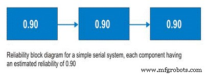
Figure 9. Simple Serial System

Parallel Systems
Often, design engineers will incorporate redundancy into critical machines. Reliability engineers call these parallel systems. These systems may be designed as active parallel systems or standby parallel systems. The block diagram for a simple two component parallel system is shown in Figure 10.

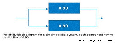
Figure 10. Simple parallel system – the system reliability is increased to 99% due to the redundancy.

To calculate the reliability of an active parallel system, where both machines are running, use the following simple equation:

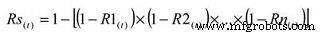
Where:
Rs(t) – System reliability for given time (t)
R1-n(t) – Subsystem or sub-function reliability for given time (t)

The simple parallel system in our example with two components in parallel, each having a reliability of 0.90, has a total system reliability of 1 – (0.1 X 0.1) =0.99. So, the system reliability was significantly improved.

There are some shortcut methods for calculating parallel system reliability when all subsystems have the same estimated reliability. More often, systems contain parallel and serial subcomponents as depicted in Figure 11. The calculation of standby systems requires knowledge about the reliability of the switching mechanism. In the interest of simplicity and brevity, this topic will be reserved for a future article.

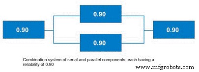
Figure 11. Combination System with Parallel and Serial Elements

r out of n Systems (r/n Systems)
An important concept to plant reliability engineers is the concept of r/n systems. These systems require that r units from a total population in n be available for use. A great industrial example is coal pulverizers in an electric power generating plant. Often, the engineers design this function in the plant using an r/n approach. For instance, a unit has four pulverizers and the unit requires that three of the four be operable to run at the unit’s full load (see Figure 12).

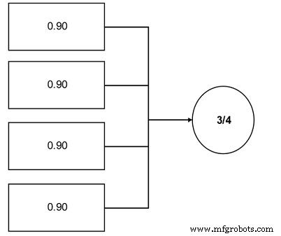
Figure 12. Simple r/n system example – Three of the four components are required.

The reliability calculation for an r/n system can be reduced to a simple cumulative binomial distribution calculation, the formula for which is:

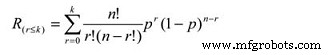
Where:
Rs =System reliability given the actual number of failures (r) is less than or equal the maximum allowable (k)
r =The actual number of failures
k =The maximum allowable number of failures
n =The total number of units in the system
p =The probability of survival, or the subcomponent reliability for a given time (t).

This equation is somewhat more complicated. In our pulverizer example, assuming a subcomponent reliability of 0.90, the equation works out as a summation of the following:
P(0) =0.6561
P(1) =0.2916

So, the likelihood of completing the mission time (t) is 0.9477 (0.6561 + 0.2916), or approximately 95%.

Field Data Collection
To employ the reliability analysis methods described herein, the engineer requires data. It is imperative to establish field data collection systems to support your reliability management initiatives. Likewise, as much as possible, you’ll want to employ common nomenclature and units so that your data can be parsed effectively for more detailed analysis. Collect the following information:

• Basic System Information
• Operating Context
• Environmental Context
• Failure Data

A good general system for data collection is described in the IEC standard 300-3-2. In addition to providing instructions for collecting field data, it provides a standard taxonomy of failure modes. Other taxonomies have been established, but the IEC standard represents a good starting point for your organization to define its own. Likewise, DOE standard NE-1004-92 offers a very nice standard nomenclature of failure causes.

An important benefit derived from your efforts to collect good field data is that it enables you to break the “random trap.” As I mentioned earlier, the bathtub curve has been much maligned – particularly in the Reliability-Centered Maintenance literature. While it’s true that Weibull analysis reveals that few complex mechanical systems exhibit time-dependent wearout failures, the reason, at least in part, is due to the fact that the reliability of complex systems is affected by a wide variety of failure modes and mechanisms.

When these are lumped together, there is a “randomizing” effect, which makes the failures appear to lack any time dependency. However, if the failure modes were analyzed individually, the story would likely be very different (Figure 13). For certain, some failure modes would still be mathematically random, but many, and arguably most, would exhibit a time dependency. This kind of information would arm reliability engineers and managers with a powerful set of options for mitigating failure risk with a high degree of precision. Naturally, this ability depends upon the effective collection and subsequent analysis of field data.

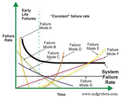
Figure 13. Good field data collection enables you to break the random trap.

This brief introduction to reliability engineering methods is intended to expose the otherwise uninitiated plant engineer to the world of quantitative reliability engineering. The subject is quite broad, however, and I’ve only touched on the major reliability methods that I believe are most applicable to the plant engineer. I encourage you to further investigate the field of reliability engineering methods, concentrating on the following topics, among others:

• More detailed understanding of the Weibull distribution and its applications

• More detailed understanding of the exponential distribution and its applications

• The Gaussian distribution and its applications

• The log-normal distribution and its applications

• Confidence intervals (binomial, chi-square/Poisson, etc.)

• Beta distribution and its applications

• Bayesian applications of reliability engineering methods

• Stress-strength interference analysis

• Testing options and their applicability to plant reliability engineering

• Reliability growth strategies and management

• More detailed understanding of field data collection.

Most important, spend time learning how to apply reliability engineering methods to plant reliability problems. If your interest in reliability engineering methods is high, I encourage you to pursue professional certification by the American Society for Quality as a reliability engineer (CRE).

References
Troyer, D. (2006) Strategic Plant Reliability Management Course Book, Noria Publishing, Tulsa, Oklahoma.

Bernowski, K (1997) “Safety in the Skies,” Quality Progress , January.

Dovich, R. (1990) Reliability Statistics, ASQ Quality Press, Milwaukee, WI.

Krishnamoorthi, K.S. (1992) Reliability Methods for Engineers, ASQ Quality Press , Milwaukee, WI.

MIL Standard 721

IEC Standard 300-3-3

DOE Standard NE-1004-92

Appendix:Select reliability engineering terms from MIL STD 721
Availability – A measure of the degree to which an item is in the operable and committable state at the start of the mission, when the mission is called for at an unknown state.

Capability – A measure of the ability of an item to achieve mission objectives given the conditions during the mission.

Dependability – A measure of the degree to which an item is operable and capable of performing its required function at any (random) time during a specified mission profile, given the availability at the start of the mission.

Failure – The event, or inoperable state, in which an item, or part of an item, does not, or would not, perform as previously specified.

Failure, dependent – Failure which is caused by the failure of an associated item(s). Not independent.

Failure, independent – Failure which occurs without being caused by the failure of any other item. Not dependent.

Failure mechanism – The physical, chemical, electrical, thermal or other process which results in failure.

Failure mode – The consequence of the mechanism through which the failure occurs, i.e. short, open, fracture, excessive wear.

Failure, random – Failure whose occurrence is predictable only in the probabilistic or statistical sense. This applies to all distributions.

Failure rate – The total number of failures within an item population, divided by the total number of life units expended by that population, during a particular measurement interval under stated conditions.

Maintainability – The measure of the ability of an item to be retained or restored to specified condition when maintenance is performed by personnel having specified skill levels, using prescribed procedures and resources, at each prescribed level of maintenance and repair.

Maintenance, corrective – All actions performed, as a result of failure, to restore an item to a specified condition. Corrective maintenance can include any or all of the following steps:localization, isolation, disassembly, interchange, reassembly, alignment and checkout.

Maintenance, preventive – All actions performed in an attempt to retain an item in a specified condition by providing systematic inspection, detection and prevention of incipient failures.

Mean time between failure (MTBF) – A basic measure of reliability for repairable items:the mean number of life units during which all parts of the item perform within their specified limits, during a particular measurement interval under stated conditions.

Mean time to failure (MTTF) – A basic measure of reliability for non-repairable items:The mean number of life units during which all parts of the item perform within their specified limits, during a particular measurement interval under stated conditions.

Mean time to repair (MTTR) – A basic measure of maintainability:the sum of corrective maintenance times at any specified level of repair, divided by the total number of failures within an item repaired at that level, during a particular interval under stated conditions.

Mission reliability – The ability of an item to perform its required functions for the duration of specified mission profile.

Reliability – (1) The duration or probability of failure-free performance under stated conditions. (2) The probability that an item can perform its intended function for a specified interval under stated conditions. For non-redundant items this is the equivalent to definition (1). For redundant items, this is the definition of mission reliability.