多相电力系统中的谐波

在关于混合频率信号的章节中，我们探讨了谐波的概念 在交流系统中：频率是基本源频率的整数倍。

在交流电源系统中，来自交流发电机（交流发电机）的电源电压波形应该是单频正弦波，没有失真，应该没有谐波成分。 . .理想情况下。

交流系统上的非线性分量

如果不是非线性分量，这将是正确的 .非线性元件会与源电压不成比例地汲取电流，从而导致非正弦电流波形。

非线性元件的例子包括气体放电灯、半导体功率控制器件（二极管、晶体管、SCR、TRIAC）、变压器（由于铁芯的 B/H 饱和曲线，初级绕组磁化电流通常是非正弦的），以及电动机（同样，当电动机核心内的磁场接近饱和水平时）。

即使是白炽灯也会产生轻微的非正弦电流，因为由于温度的快速波动，灯丝电阻在整个循环过程中都会发生变化。

正如我们在混合频率章节中学到的，any 否则正弦波形的失真构成谐波频率的存在。

当所讨论的非正弦波形在其平均中心线上下对称时，谐波频率仅为基频的奇数整数倍，没有偶数整数倍。

大多数非线性负载都会产生这样的电流波形，因此大多数交流电力系统中不存在偶数次谐波（2次、4次、6次、8次、10次、12次等）或仅存在极少。

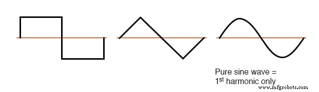
对称波形示例 - 仅奇次谐波。

下图显示了存在偶次谐波的非对称波形示例，以供参考。

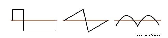
非对称波形示例 - 存在偶次谐波。

尽管非线性负载的典型对称失真消除了一半可能的谐波频率，但奇次谐波仍然会引起问题。其中一些问题对所有电力系统都是普遍存在的，无论是单相还是其他。

例如，由于涡流损耗导致的变压器过热可能发生在任何 谐波含量较大的交流电力系统。

然而，谐波电流引起的一些问题是多相电力系统特有的，本节专门针对这些问题。

关于谐波效应的 SPICE 仿真

能够在SPICE中模拟非线性负载有助于避免大量复杂的数学运算，更直观地了解谐波效应。

线性交流系统仿真

首先，我们将从一个非常简单的交流电路开始我们的模拟：一个带有纯线性负载和所有相关电阻的正弦波电压源：

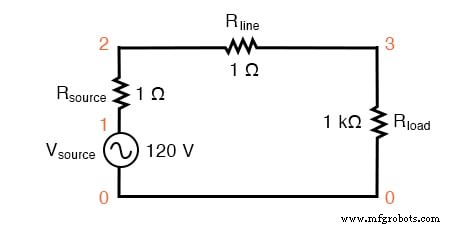
具有单个正弦波源的 SPICE 电路。

该电路中的 Rsource 和 Rline 电阻不仅仅是模拟现实世界：它们还提供方便的分流电阻，用于在 SPICE 仿真中测量电流：通过读取 1 Ω 电阻两端的电压，您可以获得通过它的电流的直接指示，因为 E =IR。

该电路的 SPICE 仿真（SPICE 列表：“线性负载仿真”）对 Rline 上测得的电压进行傅立叶分析，应该可以向我们显示该电路线路电流的谐波含量。由于本质上是完全线性的，我们应该期望没有除 60 Hz 的 1 次（基本）以外的谐波，假设是 60 Hz 源。

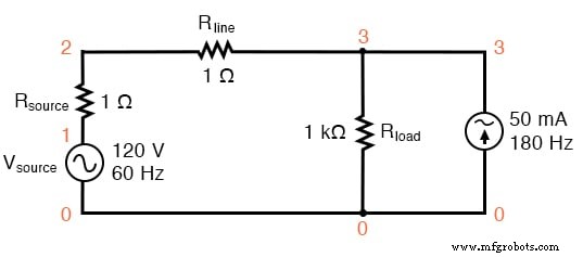
参见 SPICE 输出“瞬态响应的傅立叶分量 v(2,3)”和下图。

线性负载模拟 vsource 1 0 sin(0 120 60 0 0) 资源 1 2 1 线 2 3 1 加载 3 0 1k .options itl5=0 .tran 0.5m 30m 0 1u .plot tran v(2,3) .四 60 v(2,3) 。结尾 

<前> 瞬态响应的傅立叶分量 v(2,3) 直流分量 =4.028E-12 谐波频率 傅里叶归一化 相位归一化 无 (hz) 分量 分量 (deg) 相位 (deg) 1 6.000E+01 1.198E-01 1.000000 -72.000 0.000 2 1.200E+02 5.793E-12 0.000000 51.122 123.122 3 1.800E+02 7.407E-12 0.000000 -34.624 37.376 4 2.400E+02 9.056E-12 0.000000 4.267 76.267 5 3.000E+02 1.651E-11 0.000000 -83.461 -11.461 6 3.600E+02 3.931E-11 0.000000 36.399 108.399 7 4.200E+02 2.338E-11 0.000000 -41.343 30.657 8 4.800E+02 4.716E-11 0.000000 53.324 125.324 9 5.400E+02 3.453E-11 0.000000 21.691 93.691 总谐波失真 =0.000000%

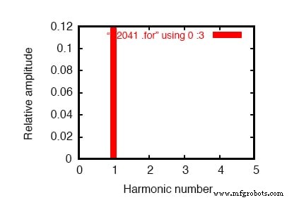
单频分量的频域图。请参阅 SPICE 列表：“线性负载模拟”。

.plot 命令出现在 SPICE 网表中，通常这会产生正弦波图输出。然而，在这种情况下，为了简洁起见，我特意省略了波形显示——.plot 命令在网表中只是为了满足 SPICE 的傅立叶变换函数的一个怪癖。

没有任何离散傅立叶变换是完美的，因此我们看到对于直到第 9 次谐波（在表中）的所有频率都指示出非常小的谐波电流（在皮安范围内！），这是 SPICE 在执行傅立叶分析时所做的.

我们显示 0.1198 安培 (1.198E-01) 的 1 次谐波或基频的“傅立叶分量”，这是我们预期的负载电流：大约 120 mA，假设电源电压为 120 伏，负载电阻为 1千欧。

简单的非线性单相交流系统仿真

接下来，我想模拟一个非线性负载以产生谐波电流。这可以通过两种根本不同的方式来完成。一种方法是使用非线性元件设计负载，例如二极管或其他易于使用 SPICE 仿真的半导体器件。另一种是在负载电阻上并联一些交流电流源。

工程师通常更喜欢使用后一种方法来模拟谐波，因为与具有高度复杂响应特性的组件相比，已知值的电流源更适合于数学网络分析。

由于我们让 SPICE 完成所有数学工作，半导体组件的复杂性不会给我们带来麻烦，但是由于可以微调电流源以产生任意数量的电流（一个方便的功能），我将选择下图所示的后一种方法，并在 SPICE 列表“非线性负载仿真”中。

SPICE 电路：添加 3 次谐波的 60 Hz 源。

<前> 非线性负载模拟 vsource 1 0 sin(0 120 60 0 0) 资源 1 2 1 线 2 3 1 加载 3 0 1k i3har 3 0 sin(0 50m 180 0 0) .options itl5=0 .tran 0.5m 30m 0 1u .plot tran v(2,3) .四 60 v(2,3) 。结尾

在这个电路中，我们有一个 50 mA 幅度的电流源和 180 Hz 的频率，这是 60 Hz 源频率的三倍。与1 kΩ负载电阻并联，其电流将与电阻相加，形成非正弦总线路电流。

我将在下图中显示波形图，以便您可以看到这个 3 次谐波电流对总电流的影响，总电流通常是一个简单的正弦波。

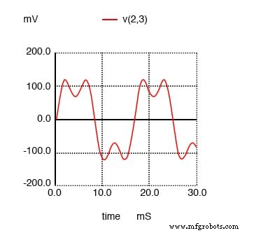
SPICE 时域图显示了 60 Hz 源和 180 Hz 的 3 次谐波之和。

瞬态响应的傅立叶分量 v(2,3) 直流分量 =1.349E-11 谐波频率 傅里叶归一化 相位归一化 无 (hz) 分量 分量 (deg) 相位 (deg) 1 6.000E+01 1.198E-01 1.000000 -72.000 0.000 2 1.200E+02 1.609E-11 0.000000 67.570 139.570 3 1.800E+02 4.990E-02 0.416667 144.000 216.000 4 2.400E+02 1.074E-10 0.000000 -169.546 -97.546 5 3.000E+02 3.871E-11 0.000000 169.582 241.582 6 3.600E+02 5.736E-11 0.000000 140.845 212.845 7 4.200E+02 8.407E-11 0.000000 177.071 249.071 8 4.800E+02 1.329E-10 0.000000 156.772 228.772 9 5.400E+02 2.619E-10 0.000000 160.498 232.498 总谐波失真 =41.666663% 

SPICE 傅立叶图显示 60 Hz 源和 180 Hz 的 3 次谐波。

在傅里叶分析中，（参见上图和“瞬态响应的傅里叶分量 v(2,3)”）混合频率未混合并单独呈现。

在这里，我们看到与第一次模拟中相同的 0.1198 安培 60 Hz（基本）电流，但出现在 3 次谐波行中，我们看到 49.9 mA：我们的 50 mA、180 Hz 电流源在工作。为什么我们看不到整个 50 mA 通过线路？

由于该电流源跨接在 1 kΩ 负载电阻器上，因此其部分电流通过负载分流而不会通过线路返回到电源。这是这种模拟的必然结果，其中一部分负载“正常”（电阻），另一部分被电流源模拟。

具有多个电流源的非线性单相交流系统仿真

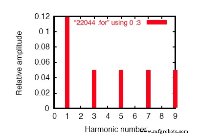
如果我们向“负载”添加更多电流源，我们会看到线电流波形与理想正弦波形的进一步失真，并且这些谐波电流中的每一个都会出现在傅立叶分析击穿中。参见下图和 SPICE 列表：“非线性负载模拟”。

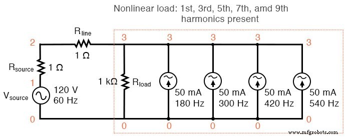
非线性负载：存在 1 次、3 次、5 次、7 次和 9 次谐波。

非线性负载模拟 vsource 1 0 sin(0 120 60 0 0) 资源 1 2 1 线 2 3 1 加载 3 0 1k i3har 3 0 sin(0 50m 180 0 0) i5har 3 0 sin(0 50m 300 0 0) i7har 3 0 sin(0 50m 420 0 0) i9har 3 0 sin(0 50m 540 0 0) .options itl5=0 .tran 0.5m 30m 0 1u .plot tran v(2,3) .四 60 v(2,3) .end 

瞬态响应的傅立叶分量 v(2,3) 直流分量 =6.299E-11 谐波频率 傅里叶归一化 相位归一化 无 (hz) 分量 分量 (deg) 相位 (deg) 1 6.000E+01 1.198E-01 1.000000 -72.000 0.000 2 1.200E+02 1.900E-09 0.000000 -93.908 -21.908 3 1.800E+02 4.990E-02 0.416667 144.000 216.000 4 2.400E+02 5.469E-09 0.000000 -116.873 -44.873 5 3.000E+02 4.990E-02 0.416667 0.000 72.000 6 3.600E+02 6.271E-09 0.000000 85.062 157.062 7 4.200E+02 4.990E-02 0.416666 -144.000 -72.000 8 4.800E+02 2.742E-09 0.000000 -38.781 33.219 9 5.400E+02 4.990E-02 0.416666 72.000 144.000 总谐波失真 =83.333296% 

傅立叶分析：“瞬态响应的傅立叶分量 v(2,3)”。

正如您从傅立叶分析（上图）中看到的，每个谐波电流源在线路电流中均等表示，每个为 49.9 mA。到目前为止，这只是一个单相电力系统仿真。

三相交流系统仿真

当我们将其设为三相模拟时，事情会变得更有趣。将执行两种傅立叶分析：一种用于线路电阻器两端的电压，一种用于中性电阻器两端的电压。

和以前一样，读取每个 1 Ω 固定电阻上的电压可以直接指示通过这些电阻的电流。参见下图和 SPICE 列表“带谐波的 Y-Y 源/负载 4 线系统”。

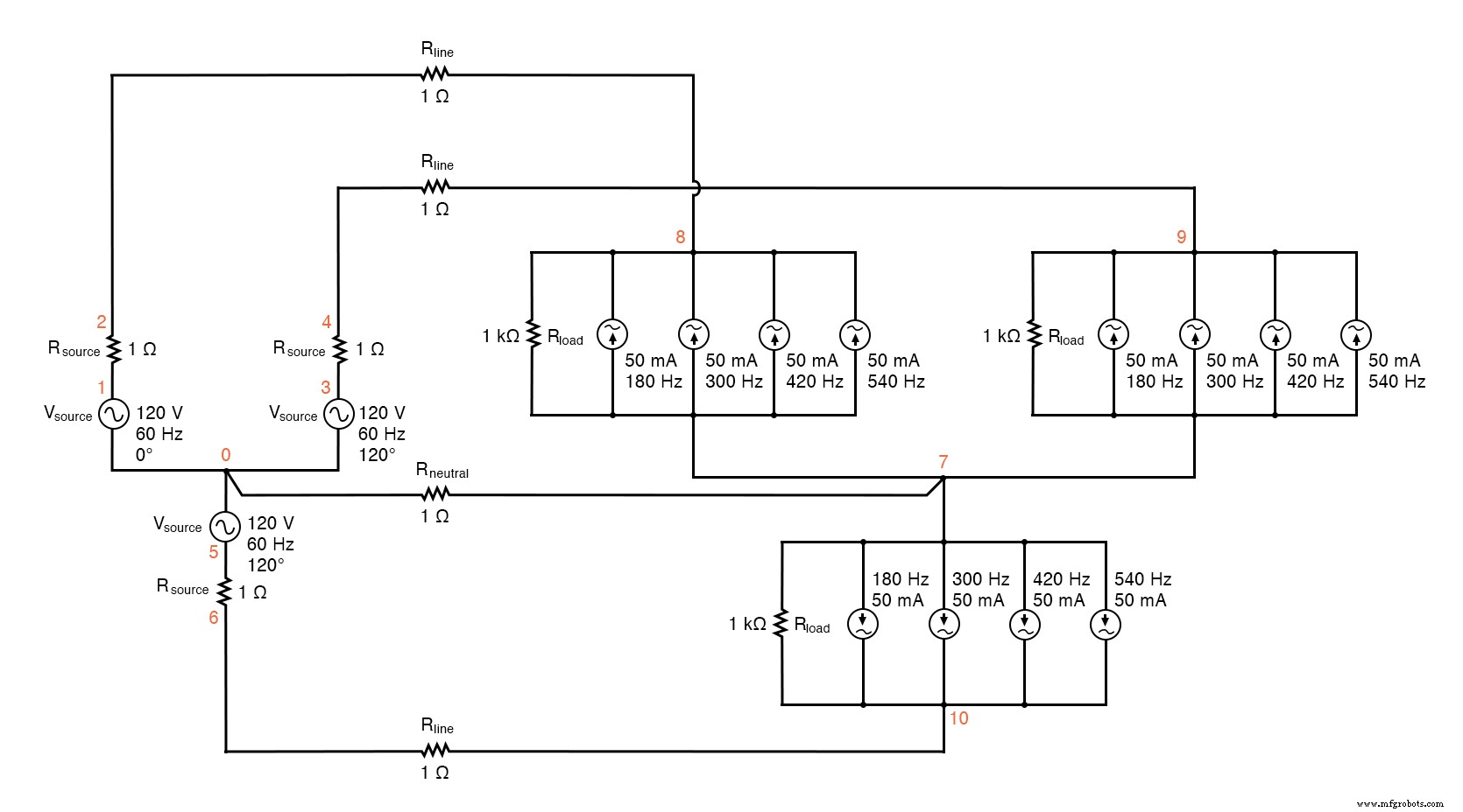
SPICE 电路：分析“线电流”和“中性线电流”，带谐波的 Y-Y 源/负载 4 线系统。

带谐波的Y-Y源/负载4线系统 * * phase1 电压源和 r (120 v /_ 0 deg) vsource1 1 0 sin(0 120 60 0 0) 资源1 1 2 1 * * phase2 电压源和 r (120 v /_ 120 deg) vsource2 3 0 sin(0 120 60 5.55555m 0) 资源 2 3 4 1 * * phase3 电压源和 r (120 v /_ 240 deg) vsource3 5 0 sin(0 120 60 11.1111m 0) 资源 3 5 6 1 * * 线路和零线电阻 rline1 2 8 1 rline2 4 9 1 rline3 6 10 1 中性 0 7 1 * * 负载的第 1 阶段 rload1 8 7 1k i3har1 8 7 sin(0 50m 180 0 0) i5har1 8 7 sin(0 50m 300 0 0) i7har1 8 7 sin(0 50m 420 0 0) i9har1 8 7 sin(0 50m 540 0 0) * * 负载的第 2 阶段 rload2 9 7 1k i3har2 9 7 sin(0 50m 180 5.55555m 0) i5har2 9 7 sin(0 50m 300 5.55555m 0) i7har2 9 7 sin(0 50m 420 5.55555m 0) i9har2 9 7 sin(0 50m 540 5.55555m 0) * * 负载的第 3 阶段 rload3 10 7 1k i3har3 10 7 sin(0 50m 180 11.1111m 0) i5har3 10 7 sin(0 50m 300 11.1111m 0) i7har3 10 7 sin(0 50m 420 11.1111m 0) i9har3 10 7 sin(0 50m 540 11.1111m 0) * * 分析的东西 .options itl5=0 .tran 0.5m 100m 12m 1u .plot tran v(2,8) .四 60 v(2,8) .plot tran v(0,7) .四 60 v(0,7) 。结尾 

线电流的傅里叶分析：

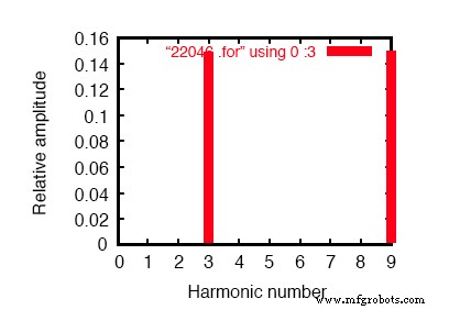
瞬态响应的傅立叶分量 v(2,8) 直流分量 =-6.404E-12 谐波频率 傅里叶归一化 相位归一化 无 (hz) 分量 分量 (deg) 相位 (deg) 1 6.000E+01 1.198E-01 1.000000 0.000 0.000 2 1.200E+02 2.218E-10 0.000000 172.985 172.985 3 1.800E+02 4.975E-02 0.415423 0.000 0.000 4 2.400E+02 4.236E-10 0.000000 166.990 166.990 5 3.000E+02 4.990E-02 0.416667 0.000 0.000 6 3.600E+02 1.877E-10 0.000000 -147.146 -147.146 7 4.200E+02 4.990E-02 0.416666 0.000 0.000 8 4.800E+02 2.784E-10 0.000000 -148.811 -148.811 9 5.400E+02 4.975E-02 0.415422 0.000 0.000 总谐波失真 =83.209009% 

平衡Y-Y系统线路电流的傅里叶分析。

中性电流的傅里叶分析：

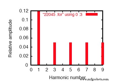
瞬态响应的傅立叶分量 v(0,7) 直流分量 =1.819E-10 谐波频率 傅里叶归一化 相位归一化 无 (hz) 分量 分量 (deg) 相位 (deg) 1 6.000E+01 4.337E-07 1.000000 60.018 0.000 2 1.200E+02 1.869E-10 0.000431 91.206 31.188 3 1.800E+02 1.493E-01 344147.7638 -180.000 -240.018 4 2.400E+02 1.257E-09 0.002898 -21.103 -81.121 5 3.000E+02 9.023E-07 2.080596 119.981 59.963 6 3.600E+02 3.396E-10 0.000783 15.882 -44.136 7 4.200E+02 1.264E-06 2.913955 59.993 -0.025 8 4.800E+02 5.975E-10 0.001378 35.584 -24.434 9 5.400E+02 1.493E-01 344147.4889 -179.999 -240.017 

中性线电流的傅立叶分析显示除了没有谐波之外！与上图中的线电流相比。

这是一个平衡的 Y-Y 电源系统，每一相都与之前模拟的单相交流系统相同。因此，三相系统中一相线电流的傅立叶分析与单相系统中线电流的傅立叶分析几乎相同也就不足为奇了：基波 (60 Hz) 线电流为0.1198 安培和每个约 50 mA 的奇次谐波电流。

见上图和傅立叶分析：“瞬态响应的傅立叶分量v(2,8)”

这里应该令人惊讶的是对中性导体电流的分析，这是由 SPICE 节点 0 和 7 之间的 Rneutral 电阻器上的电压降确定的。

在平衡的三相 Y 负载中，我们预计中性线电流为零。每相电流（其本身将通过中性线返回源 Y 上的供电相）应该在中性导体方面相互抵消，因为它们的幅度相同，并且都相隔 120°。

在没有谐波电流的系统中，这是 会发生什么，通过中性导体留下零电流。

系统中谐波电流的影响

但是，我们不能对 harmonic 说同样的话 同一系统中的电流。

请注意，中性导体中几乎没有基频（60 Hz，或 1 次谐波）电流。我们的傅立叶分析显示，读取 Rneutral 两端的电压时，一阶谐波仅为 0.4337 µA。对于 5 次和 7 次谐波也可以这样说，这两个电流的幅度都可以忽略不计。

相比之下，中性导体中的 3 次和 9 次谐波强烈表现出来，每个 149.3 mA（1 Ω 上的 1.493E-01 伏特）！这非常接近 150 mA，或电流源值的三倍。

负载中每个谐波频率有三个源，看起来我们每相中的 3 次和 9 次谐波电流相加 形成中性电流。参见傅立叶分析：“瞬态响应的傅立叶分量 v(0,7) ”

时域图分析

这正是正在发生的事情，尽管可能不清楚为什么会这样。

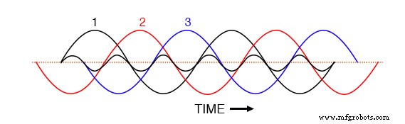
理解这一点的关键在相电流的时域图中很清楚。检查此平衡相电流随时间变化的图，相序为 1-2-3。 （下图）

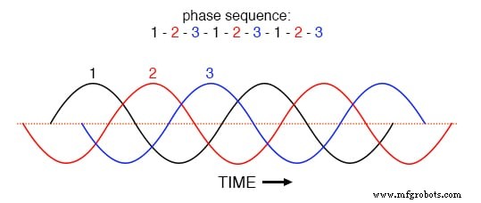
等距波的相序 1-2-3-1-2-3-1-2-3。

由于三个基本波形在图表的时间轴上均等地移动，很容易看出它们如何相互抵消以在中性导体中产生零电流。不过，让我们考虑一下，相 1 的 3 次谐波波形叠加在下图中的图形上会是什么样子。

叠加在三相基波上的第 1 相三次谐波波形。

观察这个谐波波形如何与第 2 和第 3 基波波形具有相同的相位关系，就像它与第 1 次一样：在 any 的每个正半周期中 在基波波形中，您会发现谐波波形正好有两个正半周和一个负半周。

这意味着三个 120° 相移基频波形的 3 次谐波波形实际上同相 彼此。三相交流系统中一般假设的120°相移数字仅适用于基频，不适用于其谐波倍数！

如果我们在同一张图上绘制所有三个 3 次谐波波形，我们会看到它们精确重叠并显示为一个单一的、统一的波形（在（下图）中以粗体显示

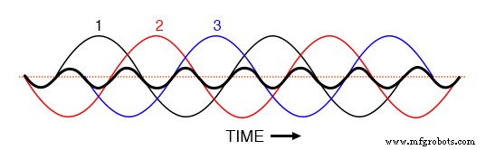
相 1、2、3 的三次谐波叠加在三相基本波形上时全部重合。

时域图的数学分析

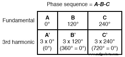
对于更倾向于数学的人来说，这个原则可以象征性地表达。假设 A 代表一个波形和B 另一个，两者频率相同，但相位相差 120°。让我们称每个波形的 3 次谐波 A' 和 B' , 分别。

A’之间的相移 和 B' 不是 120°（即 A 之间的相移 和 B )，但 3 倍，因为 A' 和 B' 波形交替速度是 A 的三倍 和 B .波形之间的偏移仅用相角准确表示 假设角速度相同时。

当关联不同频率的波形时，最准确的表示相移的方法是时间;和时移 A’之间 和 B' 相当于以低三倍的频率为 120°，或以 A’ 的频率为 360° 和 B' . 360°的相移与0°的相移是一样的，也就是说完全没有相移。

因此，A’ 和 B' 必须彼此同步：

三相系统中三次谐波的这种特性也适用于三次谐波的任何整数倍。

因此，不仅每个基波的 3 次谐波波形彼此同相，而且 6 次谐波、9 次谐波、12 次谐波、15 次谐波、18 次谐波、21 次谐波等也是如此。

由于在波形失真关于中心线对称的系统中只出现奇次谐波——并且大多数非线性负载会产生对称失真——3 次谐波（6 次、12 次、18 次等）的偶数倍通常不显着，只留下奇数倍数（第 3 次、第 9 次、第 15 次、第 21 次等）对中性线电流有显着贡献。

在具有除三相之外的某些相数的多相电力系统中，这种效应发生在具有相同倍数的谐波中。例如，在基波之间的相移为 90°的星形连接的四相系统的中性导体中添加的谐波电流将是第 4 次、第 8 次、第 12 次、第 16 次、第 20 次等。

三次谐波

由于其在三相电力系统中的丰富性和重要性，三次谐波及其倍数有自己的特殊名称：triplelen Harmons .

所有三重谐波在 4 线 Y 型连接负载的中性导体中相互叠加。在包含大量非线性负载的电力系统中，三重谐波电流可能大到足以导致中性导体过热。

这是非常有问题的，因为其他安全问题禁止中性导体具有过电流保护，因此没有提供自动中断这些高电流的规定。

分析 Y-Y 电路中三次谐波的影响

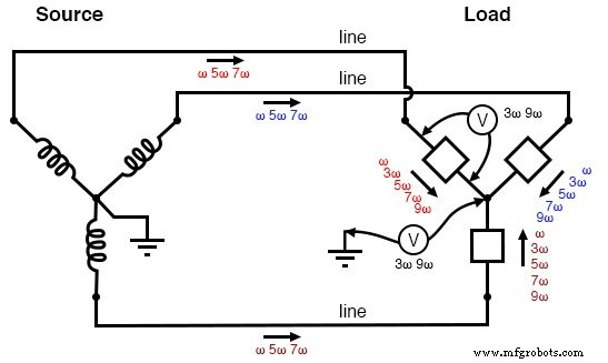
下图显示了负载产生的三倍谐波电流如何添加到中性导体中。符号“ω”用于表示角速度，在数学上等同于 2πf。所以，“ω”代表基频，“3ω”代表三次谐波，“5ω”代表五次谐波，依此类推：（下图）

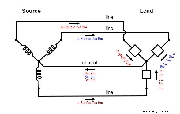
“Y-Y”三重源/负载：谐波电流添加到中性导体中。

为了减轻这些附加的三重电流，人们可能会想要完全移除中性线。如果没有中性线可以让三重电流一起流动，那么它们就不会，对吗？

不幸的是，这样做只会导致一个不同的问题：负载的“Y”中心点将不再与源的电位相同，这意味着负载的每一相将接收到与源产生的电压不同的电压。

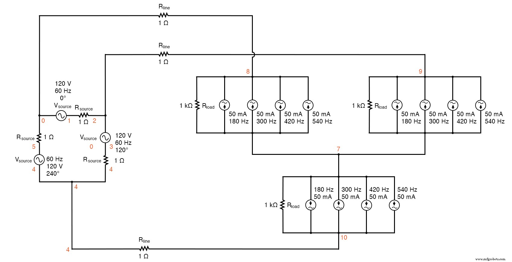
我们将在没有 1 Ω Rneutral 电阻的情况下重新运行上一次 SPICE 仿真，看看会发生什么：

带谐波的 Y-Y 源/负载（无中线） * * phase1 voltage source and r (120 v / 0 deg) vsource1 1 0 sin(0 120 60 0 0) rsource1 1 2 1 * * phase2 voltage source and r (120 v / 120 deg) vsource2 3 0 sin(0 120 60 5.55555m 0) rsource2 3 4 1 * * phase3 voltage source and r (120 v / 240 deg) vsource3 5 0 sin(0 120 60 11.1111m 0) rsource3 5 6 1 * * line resistances rline1 2 8 1 rline2 4 9 1 rline3 6 10 1 * * phase 1 of load rload1 8 7 1k i3har1 8 7 sin(0 50m 180 0 0) i5har1 8 7 sin(0 50m 300 0 0) i7har1 8 7 sin(0 50m 420 0 0) i9har1 8 7 sin(0 50m 540 0 0) * * phase 2 of load rload2 9 7 1k i3har2 9 7 sin(0 50m 180 5.55555m 0) i5har2 9 7 sin(0 50m 300 5.55555m 0) i7har2 9 7 sin(0 50m 420 5.55555m 0) i9har2 9 7 sin(0 50m 540 5.55555m 0) * * phase 3 of load rload3 10 7 1k i3har3 10 7 sin(0 50m 180 11.1111m 0) i5har3 10 7 sin(0 50m 300 11.1111m 0) i7har3 10 7 sin(0 50m 420 11.1111m 0) i9har3 10 7 sin(0 50m 540 11.1111m 0) * * analysis stuff .options itl5=0 .tran 0.5m 100m 12m 1u .plot tran v(2,8) .four 60 v(2,8) .plot tran v(0,7) .four 60 v(0,7) .plot tran v(8,7) .four 60 v(8,7) 。结尾 

Fourier analysis of line current:

Fourier components of transient response v(2,8) dc component =5.423E-11 harmonic frequency Fourier normalized phase normalized 无 (hz) 分量 分量 (deg) 相位 (deg) 1 6.000E+01 1.198E-01 1.000000 0.000 0.000 2 1.200E+02 2.388E-10 0.000000 158.016 158.016 3 1.800E+02 3.136E-07 0.000003 -90.009 -90.009 4 2.400E+02 5.963E-11 0.000000 -111.510 -111.510 5 3.000E+02 4.990E-02 0.416665 0.000 0.000 6 3.600E+02 8.606E-11 0.000000 -124.565 -124.565 7 4.200E+02 4.990E-02 0.416668 0.000 0.000 8 4.800E+02 8.126E-11 0.000000 -159.638 -159.638 9 5.400E+02 9.406E-07 0.000008 -90.005 -90.005 total harmonic distortion =58.925539 percent 

Fourier analysis of voltage between the two “Y” center-points:

Fourier components of transient response v(0,7) dc component =6.093E-08 harmonic frequency Fourier normalized phase normalized 无 (hz) 分量 分量 (deg) 相位 (deg) 1 6.000E+01 1.453E-04 1.000000 60.018 0.000 2 1.200E+02 6.263E-08 0.000431 91.206 31.188 3 1.800E+02 5.000E+01 344147.7879 -180.000 -240.018 4 2.400E+02 4.210E-07 0.002898 -21.103 -81.121 5 3.000E+02 3.023E-04 2.080596 119.981 59.963 6 3.600E+02 1.138E-07 0.000783 15.882 -44.136 7 4.200E+02 4.234E-04 2.913955 59.993 -0.025 8 4.800E+02 2.001E-07 0.001378 35.584 -24.434 9 5.400E+02 5.000E+01 344147.4728 -179.999 -240.017 total harmonic distortion =************ percent 

Fourier analysis of load phase voltage:

Fourier components of transient response v(8,7) dc component =6.070E-08 harmonic frequency Fourier normalized phase normalized 无 (hz) 分量 分量 (deg) 相位 (deg) 1 6.000E+01 1.198E+02 1.000000 0.000 0.000 2 1.200E+02 6.231E-08 0.000000 90.473 90.473 3 1.800E+02 5.000E+01 0.417500 -180.000 -180.000 4 2.400E+02 4.278E-07 0.000000 -19.747 -19.747 5 3.000E+02 9.995E-02 0.000835 179.850 179.850 6 3.600E+02 1.023E-07 0.000000 13.485 13.485 7 4.200E+02 9.959E-02 0.000832 179.790 179.789 8 4.800E+02 1.991E-07 0.000000 35.462 35.462 9 5.400E+02 5.000E+01 0.417499 -179.999 -179.999 total harmonic distortion =59.043467 percent 

Strange things are happening, indeed.

First, we see that the triplen harmonic currents (3rd and 9th) all but disappear in the lines connecting a load to source. The 5th and 7th harmonic currents are present at their normal levels (approximately 50 mA), but the 3rd and 9th harmonic currents are of negligible magnitude.

Second, we see that there is a substantial harmonic voltage between the two “Y” center-points, between which the neutral conductor used to connect. According to SPICE, there are 50 volts of both 3rd and 9th harmonic frequency between these two points, which is definitely not normal in a linear (no harmonics), balanced Y system.

Finally, the voltage as measured across one of the load’s phases (between nodes 8 and 7 in the SPICE analysis) likewise shows strong triplen harmonic voltages of 50 volts each.

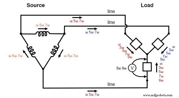
The figure below is a graphical summary of the aforementioned effects.

Three-wire “Y-Y” (no neutral) system:Triplen voltages appear between “Y” centers. Triplen voltages appear across load phases. Non-triplen currents appear in line conductors.

In summary, removal of the neutral conductor leads to a “hot” center-point on the load “Y”, and also to harmonic load phase voltages of equal magnitude, all comprised of triplen frequencies.

In the previous simulation where we had a 4-wire, Y-connected system, the undesirable effect from harmonics was excessive neutral current , but at least each phase of the load received voltage nearly free of harmonics.

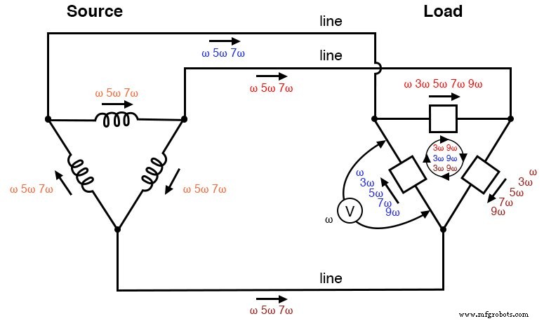
Analysis of the Effects of Triplen Harmonics in a Delta-Wye(Y) Circuit

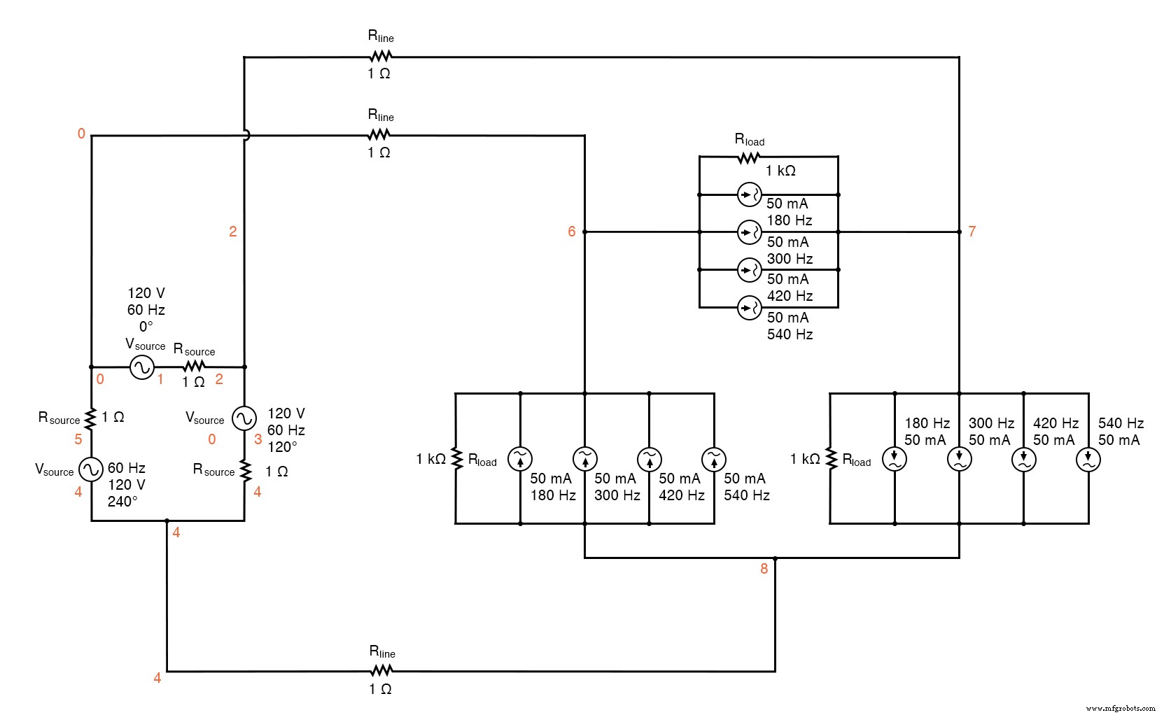
Since removing the neutral wire didn’t seem to work in eliminating the problems caused by harmonics, perhaps switching to a Δ configuration will. Let’s try a Δ source instead of a Y, keeping the load in its present Y configuration, and see what happens.

The measured parameters will be line current (voltage across Rline, nodes 0 and 8), load phase voltage (nodes 8 and 7), and source phase current (voltage across Rsource, nodes 1 and 2). （下图）

Delta-Y source/load with harmonics

Delta-Y source/load with harmonics * * phase1 voltage source and r (120 v /_ 0 deg) vsource1 1 0 sin(0 207.846 60 0 0) rsource1 1 2 1 * * phase2 voltage source and r (120 v /_ 120 deg) vsource2 3 2 sin(0 207.846 60 5.55555m 0) rsource2 3 4 1 * * phase3 voltage source and r (120 v /_ 240 deg) vsource3 5 4 sin(0 207.846 60 11.1111m 0) rsource3 5 0 1 * * line resistances rline1 0 8 1 rline2 2 9 1 rline3 4 10 1 * * phase 1 of load rload1 8 7 1k i3har1 8 7 sin(0 50m 180 9.72222m 0) i5har1 8 7 sin(0 50m 300 9.72222m 0) i7har1 8 7 sin(0 50m 420 9.72222m 0) i9har1 8 7 sin(0 50m 540 9.72222m 0) * * phase 2 of load rload2 9 7 1k i3har2 9 7 sin(0 50m 180 15.2777m 0) i5har2 9 7 sin(0 50m 300 15.2777m 0) i7har2 9 7 sin(0 50m 420 15.2777m 0) i9har2 9 7 sin(0 50m 540 15.2777m 0) * * phase 3 of load rload3 10 7 1k i3har3 10 7 sin(0 50m 180 4.16666m 0) i5har3 10 7 sin(0 50m 300 4.16666m 0) i7har3 10 7 sin(0 50m 420 4.16666m 0) i9har3 10 7 sin(0 50m 540 4.16666m 0) * * analysis stuff .options itl5=0 .tran 0.5m 100m 16m 1u .plot tran v(0,8) v(8,7) v(1,2) .four 60 v(0,8) v(8,7) v(1,2) 。结尾 

Note:the following paragraph is for those curious readers who follow every detail of my SPICE netlists. If you just want to find out what happens in the circuit, skip this paragraph!

When simulating circuits having AC sources of differing frequency and differing phase, the only way to do it in SPICE is to set up the sources with a delay time or phase offset specified in seconds. Thus, the 0° source has these five specifying figures:“(0 207.846 60 0 0)”, which means 0 volts DC offset, 207.846 volts peak amplitude (120 times the square root of three, to ensure the load phase voltages remain at 120 volts each), 60 Hz, 0 time delay, and 0 damping factor.

The 120° phase-shifted source has these figures:“(0 207.846 60 5.55555m 0)”, all the same as the first except for the time delay factor of 5.55555 milliseconds, or 1/3 of the full period of 16.6667 milliseconds for a 60 Hz waveform.

The 240° source must be time-delayed twice that amount, equivalent to a fraction of 240/360 of 16.6667 milliseconds, or 11.1111 milliseconds.

This is for the Δ-connected source. The Y-connected load, on the other hand, requires a different set of time-delay figures for its harmonic current sources, because the phase voltages in a Y load are not in phase with the phase voltages of a Δ source.

If Δ source voltages VAC, VBA, and VCB are referenced at 0°, 120°, and 240°, respectively, then “Y” load voltages VA, VB, and VC will have phase angles of -30°, 90°, and 210°, respectively.

This is an intrinsic property of all Δ-Y circuits and not a quirk of SPICE. Therefore, when I specified the delay times for the harmonic sources, I had to set them at 15.2777 milliseconds (-30°, or +330°), 4.16666 milliseconds (90°), and 9.72222 milliseconds (210°).

One final note:when delaying AC sources in SPICE, they don’t “turn on” until their delay time has elapsed, which means any mathematical analysis up to that point in time will be in error. Consequently, I set the .tran transient analysis line to hold off analysis until 16 milliseconds after the start, which gives all sources in the netlist time to engage before any analysis takes place.

The result of this analysis is almost as disappointing as the last. (Figure below) Line currents remain unchanged (the only substantial harmonic content being the 5th and 7th harmonics), and load phase voltages remain unchanged as well, with a full 50 volts of triplen harmonic (3rd and 9th) frequencies across each load component.

Source phase current is a fraction of the line current, which should come as no surprise. Both 5th and 7th harmonics are represented there, with negligible triplen harmonics:

Fourier analysis of line current:

<前> Fourier components of transient response v(0,8) dc component =-6.850E-11 harmonic frequency Fourier normalized phase normalized 无 (hz) 分量 分量 (deg) 相位 (deg) 1 6.000E+01 1.198E-01 1.000000 150.000 0.000 2 1.200E+02 2.491E-11 0.000000 159.723 9.722 3 1.800E+02 1.506E-06 0.000013 0.005 -149.996 4 2.400E+02 2.033E-11 0.000000 52.772 -97.228 5 3.000E+02 4.994E-02 0.416682 30.002 -119.998 6 3.600E+02 1.234E-11 0.000000 57.802 -92.198 7 4.200E+02 4.993E-02 0.416644 -29.998 -179.998 8 4.800E+02 8.024E-11 0.000000 -174.200 -324.200 9 5.400E+02 4.518E-06 0.000038 -179.995 -329.995 total harmonic distortion =58.925038 percent

Fourier analysis of load phase voltage:

Fourier components of transient response v(8,7) dc component =1.259E-08 harmonic frequency Fourier normalized phase normalized 无 (hz) 分量 分量 (deg) 相位 (deg) 1 6.000E+01 1.198E+02 1.000000 150.000 0.000 2 1.200E+02 1.941E-07 0.000000 49.693 -100.307 3 1.800E+02 5.000E+01 0.417222 -89.998 -239.998 4 2.400E+02 1.519E-07 0.000000 66.397 -83.603 5 3.000E+02 6.466E-02 0.000540 -151.112 -301.112 6 3.600E+02 2.433E-07 0.000000 68.162 -81.838 7 4.200E+02 6.931E-02 0.000578 148.548 -1.453 8 4.800E+02 2.398E-07 0.000000 -174.897 -324.897 9 5.400E+02 5.000E+01 0.417221 90.006 -59.995 total harmonic distortion =59.004109 percent 

Fourier analysis of source phase current:

Fourier components of transient response v(1,2) dc component =3.564E-11 harmonic frequency Fourier normalized phase normalized 无 (hz) 分量 分量 (deg) 相位 (deg) 1 6.000E+01 6.906E-02 1.000000 -0.181 0.000 2 1.200E+02 1.525E-11 0.000000 -156.674 -156.493 3 1.800E+02 1.422E-06 0.000021 -179.996 -179.815 4 2.400E+02 2.949E-11 0.000000 -110.570 -110.390 5 3.000E+02 2.883E-02 0.417440 -179.996 -179.815 6 3.600E+02 2.324E-11 0.000000 -91.926 -91.745 7 4.200E+02 2.883E-02 0.417398 -179.994 -179.813 8 4.800E+02 4.140E-11 0.000000 -39.875 -39.694 9 5.400E+02 4.267E-06 0.000062 0.006 0.186 total harmonic distortion =59.031969 percent 

“Δ-Y” source/load:Triplen voltages appear across load phases. Non-triplen currents appear in line conductors and in source phase windings.

Really, the only advantage of the Δ-Y configuration from the standpoint of harmonics is that there is no longer a center-point at the load posing a shock hazard. Otherwise, the load components receive the same harmonically-rich voltages and the lines see the same currents as in a three-wire Y system.

Analysis of the Effects of Triplen Harmonics in a Delta - Delta Circuit

If we were to reconfigure the system into a Δ-Δ arrangement, (Figure below) that should guarantee that each load component receives non-harmonic voltage, since each load phase would be directly connected in parallel with each source phase.

The complete lack of any neutral wires or “center points” in a Δ-Δ system prevents strange voltages or additive currents from occurring.

It would seem to be the ideal solution. Let’s simulate and observe, analyzing line current, load phase voltage, and source phase current. See SPICE listing:“Delta-Delta source/load with harmonics”, “Fourier analysis:Fourier components of transient response v(0,6)”, and “Fourier components of transient response v(2,1)”.

Delta-Delta source/load with harmonics.

Delta-Delta source/load with harmonics * * phase1 voltage source and r (120 v /_ 0 deg) vsource1 1 0 sin(0 120 60 0 0) rsource1 1 2 1 * * phase2 voltage source and r (120 v /_ 120 deg) vsource2 3 2 sin(0 120 60 5.55555m 0) rsource2 3 4 1 * * phase3 voltage source and r (120 v /_ 240 deg) vsource3 5 4 sin(0 120 60 11.1111m 0) rsource3 5 0 1 * * line resistances rline1 0 6 1 rline2 2 7 1 rline3 4 8 1 * * phase 1 of load rload1 7 6 1k i3har1 7 6 sin(0 50m 180 0 0) i5har1 7 6 sin(0 50m 300 0 0) i7har1 7 6 sin(0 50m 420 0 0) i9har1 7 6 sin(0 50m 540 0 0) * * phase 2 of load rload2 8 7 1k i3har2 8 7 sin(0 50m 180 5.55555m 0) i5har2 8 7 sin(0 50m 300 5.55555m 0) i7har2 8 7 sin(0 50m 420 5.55555m 0) i9har2 8 7 sin(0 50m 540 5.55555m 0) * * phase 3 of load rload3 6 8 1k i3har3 6 8 sin(0 50m 180 11.1111m 0) i5har3 6 8 sin(0 50m 300 11.1111m 0) i7har3 6 8 sin(0 50m 420 11.1111m 0) i9har3 6 8 sin(0 50m 540 11.1111m 0) * * analysis stuff .options itl5=0 .tran 0.5m 100m 16m 1u .plot tran v(0,6) v(7,6) v(2,1) i(3har1) .four 60 v(0,6) v(7,6) v(2,1) 。结尾 

Fourier analysis of line current:

Fourier components of transient response v(0,6) dc component =-6.007E-11 harmonic frequency Fourier normalized phase normalized 无 (hz) 分量 分量 (deg) 相位 (deg) 1 6.000E+01 2.070E-01 1.000000 150.000 0.000 2 1.200E+02 5.480E-11 0.000000 156.666 6.666 3 1.800E+02 6.257E-07 0.000003 89.990 -60.010 4 2.400E+02 4.911E-11 0.000000 8.187 -141.813 5 3.000E+02 8.626E-02 0.416664 -149.999 -300.000 6 3.600E+02 1.089E-10 0.000000 -31.997 -181.997 7 4.200E+02 8.626E-02 0.416669 150.001 0.001 8 4.800E+02 1.578E-10 0.000000 -63.940 -213.940 9 5.400E+02 1.877E-06 0.000009 89.987 -60.013 total harmonic distortion =58.925538 percent 

Fourier analysis of load phase voltage:

Fourier components of transient response v(7,6) dc component =-5.680E-10 harmonic frequency Fourier normalized phase normalized 无 (hz) 分量 分量 (deg) 相位 (deg) 1 6.000E+01 1.195E+02 1.000000 0.000 0.000 2 1.200E+02 1.039E-09 0.000000 144.749 144.749 3 1.800E+02 1.251E-06 0.000000 89.974 89.974 4 2.400E+02 4.215E-10 0.000000 36.127 36.127 5 3.000E+02 1.992E-01 0.001667 -180.000 -180.000 6 3.600E+02 2.499E-09 0.000000 -4.760 -4.760 7 4.200E+02 1.992E-01 0.001667 -180.000 -180.000 8 4.800E+02 2.951E-09 0.000000 -151.385 -151.385 9 5.400E+02 3.752E-06 0.000000 89.905 89.905 total harmonic distortion =0.235702 percent 

Fourier analysis of source phase current:

Fourier components of transient response v(2,1) dc component =-1.923E-12 harmonic frequency Fourier normalized phase normalized 无 (hz) 分量 分量 (deg) 相位 (deg) 1 6.000E+01 1.194E-01 1.000000 179.940 0.000 2 1.200E+02 2.569E-11 0.000000 133.491 -46.449 3 1.800E+02 3.129E-07 0.000003 89.985 -89.955 4 2.400E+02 2.657E-11 0.000000 23.368 -156.571 5 3.000E+02 4.980E-02 0.416918 -180.000 -359.939 6 3.600E+02 4.595E-11 0.000000 -22.475 -202.415 7 4.200E+02 4.980E-02 0.416921 -180.000 -359.939 8 4.800E+02 7.385E-11 0.000000 -63.759 -243.699 9 5.400E+02 9.385E-07 0.000008 89.991 -89.949 total harmonic distortion =58.961298 percent 

As predicted earlier, the load phase voltage is almost a pure sine-wave, with negligible harmonic content, thanks to the direct connection with the source phases in a Δ-Δ system.

But what happened to the triplen harmonics? The 3rd and 9th harmonic frequencies don’t appear in any substantial amount in the line current, nor in the load phase voltage, nor in the source phase current! We know that triplen currents exist because the 3rd and 9th harmonic current sources are intentionally placed in the phases of the load, but where did those currents go?

Analysis of the Effects of Triplen Harmonics in a Delta - Delta Circuit

Remember that the triplen harmonics of 120° phase-shifted fundamental frequencies are in phase with each other.

Note the directions that the arrows of the current sources within the load phases are pointing, and think about what would happen if the 3rd and 9th harmonic sources were DC sources instead.

What we would have is currently circulating within the loop formed by the Δ-connected phases . This is where the triplen harmonic currents have gone:they stay within the Δ of the load, never reaching the line conductors or the windings of the source.

These results may be graphically summarized as such in the figure below.

Δ-Δ source/load:Load phases receive undistorted sine wave voltages. Triplen currents are confined to circulate within load phases. Non-triplen currents appear in line conductors and in source phase windings.

This is a major benefit of the Δ-Δ system configuration:triplen harmonic currents remain confined in whatever set of components create them and do not “spread” to other parts of the system.

评论：

• Nonlinear components are those that draw a non-sinusoidal (non-sine-wave) current waveform when energized by a sinusoidal (sine-wave) voltage. Since any distortion of an originally pure sine-wave constitutes harmonic frequencies, we can say that nonlinear components generate harmonic currents.
• When the sine-wave distortion is symmetrical above and below the average centerline of the waveform, the only harmonics present will be odd-numbered , not even-numbered.
• The 3rd harmonic, and integer multiples of it (6th, 9th, 12th, 15th) are known as triplen harmonics. They are in phase with each other, despite the fact that their respective fundamental waveforms are 120° out of phase with each other.
• In a 4-wire Y-Y system, triplen harmonic currents add within the neutral conductor.
• Triplen harmonic currents in a Δ-connected set of components circulate within the loop formed by the Δ.

相关工作表：

• Mixed-Frequency Signals Worksheet