特殊转换器和应用

阻抗匹配

由于变压器可以将电压和电流步进到不同的水平，并且由于功率在初级和次级绕组之间等效传输，因此它们可用于将负载的阻抗“转换”到不同的水平。最后一句话值得解释一下，让我们研究一下它的意思。

负载（通常）的目的是利用它消耗的功率做一些富有成效的事情。在电阻加热元件的情况下，耗散功率的实际目的是加热某些东西。

负载设计为安全耗散一定的最大功率，但两个额定功率相等的负载不一定相同。考虑这两个 1000 瓦电阻加热元件：

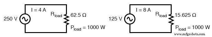
加热元件在不同的电压和电流额定值下耗散 1000 瓦。

两种加热器都消耗了 1000 瓦的功率，但它们的电压和电流水平不同（250 伏和 4 安，或 125 伏和 8 安）。使用欧姆定律确定这些加热元件的必要电阻 (R=E/I)，我们分别得出 62.5 Ω 和 15.625 Ω 的数字。

如果这些是交流负载，我们可能会用阻抗而不是简单的电阻来表示它们对电流的反对，尽管在这种情况下，这就是它们的全部组成（无电抗）。可以说 250 伏加热器的阻抗负载高于 125 伏加热器。

如果我们希望直接在 125 伏电源系统上操作 250 伏加热器元件，我们最终会感到失望。阻抗（电阻）为 62.5 Ω 时，电流仅为 2 安培（I=E/R；125/62.5），功耗仅为 250 瓦（P=IE；125 x 2），或一其额定功率的四分之一。

加热器的阻抗和我们的电源电压会不匹配，我们无法从加热器获得完整的额定功耗。

不过，并没有失去所有希望。使用升压变压器，我们可以在 125 伏电源系统上操作 250 伏加热元件，如下图所示。

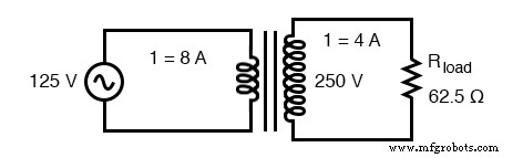
升压变压器使用 125 V 电源运行 1000 瓦 250 V 加热器。

阻抗、电流和电压变换比

变压器绕组的比率提供升压和 我们需要当前的降压，否则不匹配的负载才能在该系统上正常运行。仔细查看初级电路数字：8 安培时为 125 伏。就电源“所知”而言，它在 125 伏电压下为 15.625 Ω (R=E/I) 负载供电，而不是 62.5 Ω 负载！

初级绕组的电压和电流数字表示 15.625 Ω 负载阻抗，而不是负载本身的实际 62.5 Ω。换句话说，我们的升压变压器不仅改变了电压和电流，还改变了阻抗

阻抗变比为电压/电流变比的平方，与绕组电感比相同：

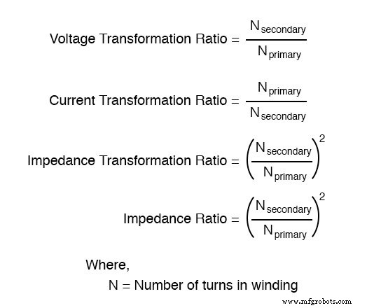
这与我们的 2:1 升压变压器示例和 62.5 Ω 到 15.625 Ω 的阻抗比（4:1 的比率，即 2:1 的平方）一致。阻抗变换是变压器的一项非常有用的能力，因为它允许负载消耗其全部额定功率，即使电力系统没有直接处于适当的电压下。

最大功率传输定理在变压器中的应用

回忆一下我们对网络分析的研究最大功率传输定理 ，这表明当负载电阻等于供电网络的戴维宁/诺顿电阻时，负载电阻将耗散最大功率。在该定义中用“阻抗”代替“电阻”，你就有了该定理的 AC 版本。

如果我们试图从负载获得理论上的最大功耗，我们必须能够将负载阻抗和源 (Thevenin/Norton) 阻抗正确匹配在一起。这通常在无线电发射器/天线和音频放大器/扬声器系统等专用电路中更受关注。

让我们以一个音频放大器系统为例，看看它是如何工作的：（下图）

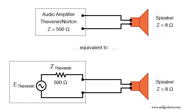
阻抗为 500 Ω 的放大器以远低于最大功率的情况驱动 8 Ω。

由于内部阻抗为 500 Ω，放大器只能向同样具有 500 Ω 阻抗的负载（扬声器）提供全功率。与耗散相同功率的 8 Ω 扬声器相比，这样的负载会降低更高的电压并消耗更少的电流。

如果如图所示将 8 Ω 扬声器直接连接到 500 Ω 放大器，阻抗不匹配 将导致非常差的（低峰值功率）性能。此外，放大器往往会以热量的形式耗散超过其公平份额的功率，以驱动低阻抗扬声器。

为了使该系统更好地工作，我们可以使用变压器来匹配这些不匹配的阻抗。由于我们要从高阻抗（高电压、低电流）电源转换为低阻抗（低电压、高电流）负载，因此我们需要使用降压变压器：

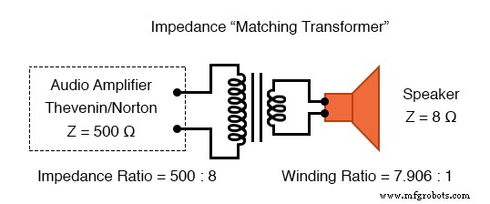
阻抗匹配变压器将 500 Ω 放大器与 8 Ω 扬声器相匹配，以获得最大效率。

阻抗匹配说明

要获得500:8的阻抗变换比，我们需要一个绕组比等于500:8的平方根（62.5:1的平方根，即7.906:1）。

有了这样的变压器，扬声器就会将放大器加载到恰到好处的程度，以正确的电压和电流水平汲取功率，以满足最大功率传输定理，并为负载提供最有效的功率传输。使用这种容量的变压器称为阻抗匹配 .

任何骑过多速自行车的人都能直观地理解阻抗匹配的原理。当以特定速度（大约每分钟 60 到 90 转）旋转自行车曲柄时，人的腿会产生最大的动力。

高于或低于该转速，人体腿部肌肉的发电效率较低。自行车“齿轮”的目的是将骑手的腿与骑行条件进行阻抗匹配，以便他们始终以最佳速度旋转曲柄。

如果骑手试图在自行车换入“最高”档时开始移动，他或她会发现很难移动。是因为骑手弱吗？

不，这是因为自行车链条和链轮的高升压比在条件（需要克服大量惯性）和它们的腿（需要以 60-90 RPM 旋转以获得最大功率输出）之间存在不匹配.

另一方面，选择太低的档位将使骑手能够立即移动，但会限制他们能够达到的最高速度。再次，缺乏速度是否表明骑自行车者的腿很虚弱？

不，这是因为所选档位的较低速比会在条件（低负载）和骑手的腿（如果旋转速度超过 90 RPM 时失去动力）之间造成另一种类型的不匹配。电源和负载也是如此：必须有阻抗匹配才能获得最大系统效率。

在交流电路中，变压器执行与自行车上的链轮和链条（“齿轮”）相同的匹配功能，以匹配其他不匹配的电源和负载。

阻抗匹配变压器

阻抗匹配变压器在结构或外观上与任何其他类型的变压器没有根本区别。用于音频应用的小型阻抗匹配变压器（宽约两厘米）如下图所示：

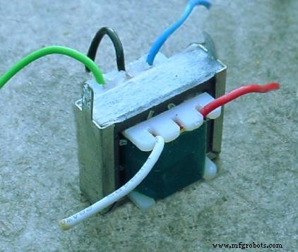
音频阻抗匹配变压器。

另一个阻抗匹配变压器可以在这个印刷电路板上看到，在右上角，电阻器 R2 和 R1 的左边。它被标记为“T1”：

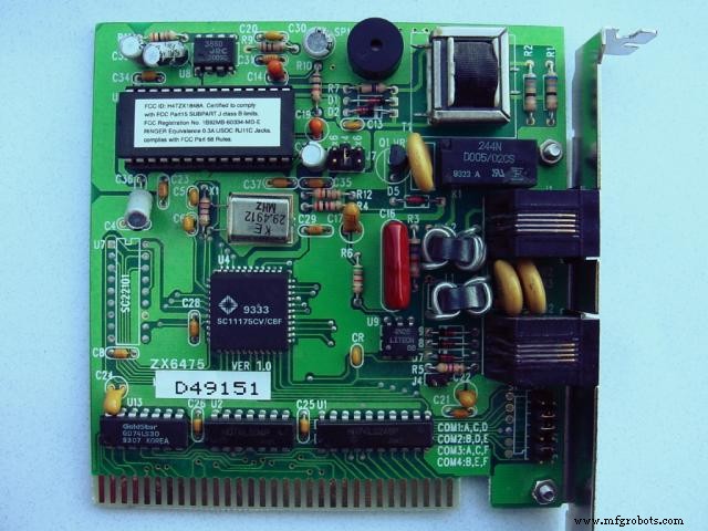
印刷电路板安装音频阻抗匹配变压器，右上角。

潜在的变形金刚

变压器也可用于电气仪表系统。由于变压器具有升高或降低电压和电流的能力，以及它们提供的电气隔离，它们可以作为将电气仪表连接到高压、大电流电源系统的一种方式。

假设我们要精确测量 13.8 kV 电力系统（美国工业中非常常见的配电电压）的电压：

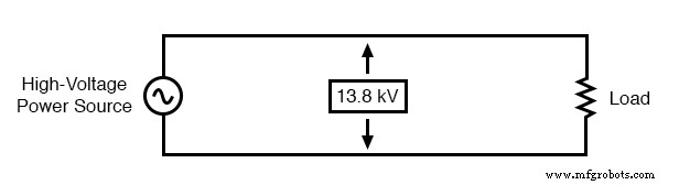
电压表直接测量高压存在安全隐患。

设计、安装和维护能够直接测量 13,800 伏交流电的电压表绝非易事。仅将 13.8 kV 导体带入仪表板的安全隐患就很严重，更不用说电压表本身的设计了。

但是，通过使用精密降压变压器，我们可以将 13.8 kV 以恒定比率降低到安全电压水平，并将其与仪器连接隔离，从而为计量系统增加额外的安全水平：

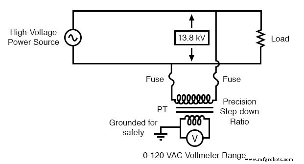
仪器应用：“电压互感器”将危险的高压精确地标定为适用于传统电压表的安全值。

现在，电压表读取实际系统电压的精确分数或比率，其刻度设置为读取，就像直接测量电压一样。

变压器将仪器电压保持在安全水平，并将其与电力系统电气隔离，因此电源线与仪器或仪器接线之间没有直接连接。当以这种容量使用时，变压器称为电位变压器 , 或者干脆PT .

电压互感器旨在提供尽可能准确的降压比。为了有助于精确的电压调节，将负载保持在最低限度：电压表采用高输入阻抗，以尽可能少地从 PT 汲取电流。

如您所见，为了安全和方便地将 PT 与电路断开，已将保险丝与 PT 初级绕组串联。

PT 的标准次级电压为 120 伏交流电，适用于全额定电源线电压。随 PT 的标准电压表量程为 150 伏，满量程。

可以制造具有定制绕组比的 PT 以适应任何应用。这非常有助于实际电压表仪器本身的行业标准化，因为 PT 的尺寸将调整为将系统电压降低到该标准仪器水平。

电流互感器

按照同样的思路，我们可以使用变压器降低通过电源线的电流，以便我们能够使用廉价的电流表安全轻松地测量高系统电流。当然，这样的变压器会与电源线串联。

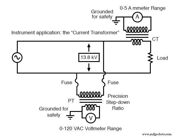
仪表应用：“电流互感器”将大电流降低到适用于传统电流表的值。

请注意，虽然 PT 是降压设备，但电流互感器 （或CT ) 是升压装置（相对于电压而言），这是降压降压所需要的 电源线电流。很多时候，CT 被构建为环形设备，电力线导体通过它运行，电力线本身充当单匝初级绕组：

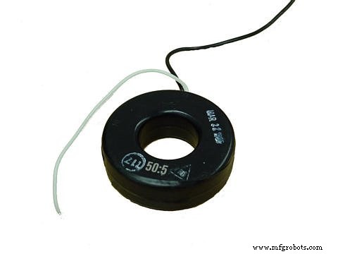
要测量的电流导体穿过开口。导线上可提供按比例缩小的电流。

一些 CT 是铰链打开的，允许在电源导体周围插入，而根本不会干扰导体。 CT 的行业标准次级电流范围为 0 到 5 安培交流电。与 PT 一样，CT 可以定制绕组比以适应几乎所有应用。

因为它们的“满载”次级电流是 5 安培，所以 CT 比通常用满载初级安培到 5 安培来描述，如下所示：

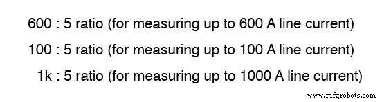
照片中的“甜甜圈”CT 的比例为 50:5。也就是说，当通过环面中心的导体承载 50 安培的电流 (AC) 时，CT 的绕组中将感应出 5 安培的电流。

因为 CT 设计用于为低阻抗负载的电流表供电，并且它们作为升压变压器绕制，所以它们永远不应该，永远 二次绕组开路运行。

不注意此警告将导致 CT 产生极高的二次电压，对设备和人员均造成危险。为方便电流表仪表的维护，短路开关通常与 CT 的次级绕组并联安装，每当电流表拆卸维修时，短路开关将闭合：

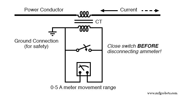
短路开关允许将电流表从有源电流互感器电路中移除。

尽管故意看起来很奇怪 将电力系统元件短路，在使用电流互感器时是完全正确和非常必要的。

空心变压器

另一种常见于射频电路中的特殊变压器是空心 变压器。顾名思义，空心变压器的绕组缠绕在非磁性形式上，通常是某种材料的空心管。

这种变压器绕组之间的耦合度（互感）比等效的铁芯变压器小很多倍，但铁磁芯的不良特性（涡流损耗、磁滞、饱和等）完全消除消除。

铁芯的这些影响在高频应用中是最成问题的。

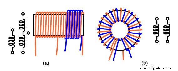
空心变压器可以缠绕在圆柱形 (a) 或环形 (b) 形式上。中心抽头初级和次级 (a)。环形双线绕组 (b)。

当不需要直流隔离时，没有过绕组的内部抽头螺线管绕组可以匹配不等阻抗。当需要隔离时，在主绕组的一端添加过绕组。空芯变压器用于射频铁芯损耗过高时。

空心变压器经常与电容器并联以将其调谐到谐振。对于此类应用，过绕组连接在无线电天线和地之间。次级通过可变电容器调谐到谐振。

输出可取自用于放大或检测的抽头点。小毫米尺寸的空心变压器用于无线电接收器。最大的无线电发射器可能使用米大小的线圈。非屏蔽空心螺线管变压器相互成直角安装，以防止杂散耦合。

当变压器绕成环形时，杂散耦合被最小化。环形空心变压器也表现出更高的耦合度，特别是对于双线 绕组。双线绕组由稍微绞合的双绞线缠绕而成。

这意味着 1:1 的匝数比。三或四根导线可以按 1:2 和其他积分比分组。绕组不必是双线的。这允许任意匝数比。然而，耦合程度受到影响。除VHF（甚高频）工作外，环形空芯变压器很少见。

铁粉或铁氧体等空气以外的磁芯材料更适合用于较低的射频。

特斯拉线圈

空心变压器的一个显着例子是特斯拉线圈 ，以塞尔维亚电气天才尼古拉特斯拉的名字命名，他也是旋转磁场交流电机、多相交流电源系统和无线电技术许多元素的发明者。

特斯拉线圈是一种谐振高频升压变压器，用于产生极高的电压。

特斯拉的梦想之一是利用他的线圈技术在不需要电线的情况下分配电力，只需以无线电波的形式广播，无线电波可以通过天线接收并传导到负载。

特斯拉线圈的基本原理图如下图所示。

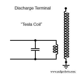
特斯拉线圈：初级匝数重，次级匝数多。

电容器与变压器的初级绕组一起形成一个储能电路。次级绕组靠近初级绕组，通常围绕相同的非磁性形式。存在多种“激励”初级电路的选项，最简单的是高压、低频交流电源和火花隙：

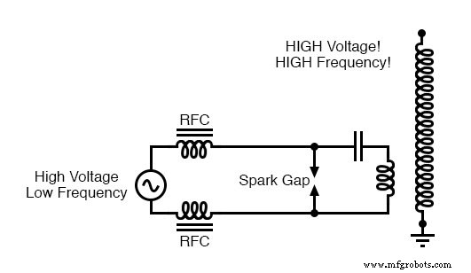
带火花隙驱动的特斯拉线圈的系统级图。

高压、低频交流电源的目的是为初级储能电路“充电”。当火花隙点火时，它的低阻抗将完成电容器/初级线圈谐振电路，使其以其谐振频率振荡。

“RFC”电感器是“射频扼流圈”，它充当高阻抗以防止交流电源干扰振荡回路。

特斯拉线圈变压器的次级侧也是一个槽路，依靠放电端和大地之间存在的寄生（杂散）电容来补充次级绕组的电感。

为了实现最佳操作，该次级槽路被调谐到与初级电路相同的谐振频率，不仅在谐振振荡期间电容器和电感器之间进行能量交换，而且在初级和次级绕组之间来回交换能量。视觉效果非常壮观：

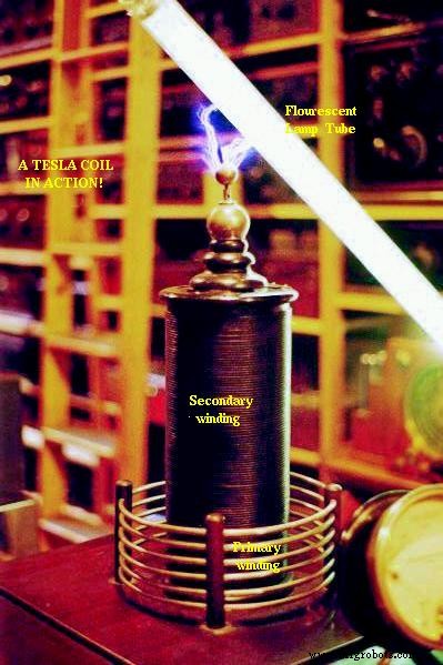
特斯拉线圈的高压高频放电。

特斯拉线圈主要用作新奇设备，出现在高中科学展、地下室研讨会和偶尔的低预算科幻电影中。

应该注意的是，特斯拉线圈可能是极其危险的设备。与所有电灼伤一样，射频 (“RF”) 电流引起的灼伤可能会很深，这与接触热物体或火焰引起的皮肤灼伤不同。

尽管特斯拉线圈的高频放电具有超出人类神经系统“震动感知”频率的奇异特性，但这并不意味着特斯拉线圈不会伤害甚至杀死您！如果您要自己动手制作，我强烈建议您寻求经验丰富的特斯拉线圈实验者的帮助。

饱和反应堆

到目前为止，我们已经探索了变压器作为一种将不同级别的电压、电流甚至阻抗从一个电路转换到另一个电路的设备。现在我们将把它看作一种完全不同的设备：一种允许小电信号施加控制的设备 在更大数量的电力上。在这种模式下，变压器充当放大器 .

我所指的设备称为饱和核心反应堆 , 或者干脆饱和反应堆 .实际上，它根本不是真正的变压器，而是一种特殊的电感器，其电感量可以通过将直流电流施加到缠绕在同一铁芯上的第二个绕组来改变。

与铁磁变压器一样，可饱和电抗器也依赖于磁饱和原理。当铁等材料完全饱和时（即其所有磁畴与施加的磁化力对齐），通过磁化绕组的电流的额外增加不会导致磁通量的进一步增加。

电感回顾

Now, inductance is the measure of how well an inductor opposes changes in current by developing a voltage in an opposing direction. The ability of an inductor to generate this opposing voltage is directly connected with the change in magnetic flux inside the inductor resulting from the change in current, and the number of winding turns in the inductor.

If an inductor has a saturated core, no further magnetic flux will result from further increases in current, and so there will be no voltage induced in opposition to the change in current. In other words, an inductor loses its inductance (ability to oppose changes in current) when its core becomes magnetically saturated.

If an inductor’s inductance changes, then its reactance (and impedance) to AC current changes as well. In a circuit with a constant voltage source, this will result in a change in current:

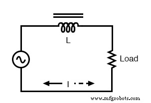
If L changes in inductance, ZL will correspondingly change, thus changing the circuit current.

Saturable Reactor Operation

A saturable reactor capitalizes on this effect by forcing the core into a state of saturation with a strong magnetic field generated by current through another winding. The reactor’s “power” winding is the one carrying the AC load current, and the “control” winding is one carrying a DC current strong enough to drive the core into saturation:

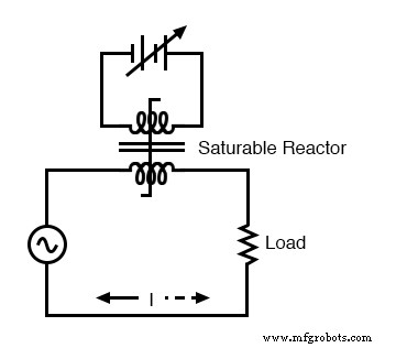
DC, via the control winding, saturates the core. Thus, modulating the power winding inductance, impedance, and current.

The strange-looking transformer symbol shown in the above schematic represents a saturable-core reactor, the upper winding being the DC control winding and the lower being the “power” winding through which the controlled AC current goes.

Increased DC control current produces more magnetic flux in the reactor core, driving it closer to a condition of saturation, thus decreasing the power winding’s inductance, decreasing its impedance, and increasing current to the load. Thus, the DC control current is able to exert control over the AC current delivered to the load.

The circuit shown would work, but it would not work very well. The first problem is the natural transformer action of the saturable reactor:AC current through the power winding will induce a voltage in the control winding, which may cause trouble for the DC power source.

Also, saturable reactors tend to regulate AC power only in one direction:in one half of the AC cycle, the mmf’s from both windings add; in the other half, they subtract. Thus, the core will have more flux in it during one half of the AC cycle than the other and will saturate first in that cycle half, passing load current more easily in one direction than the other.

Fortunately, both problems can be overcome with a little ingenuity:

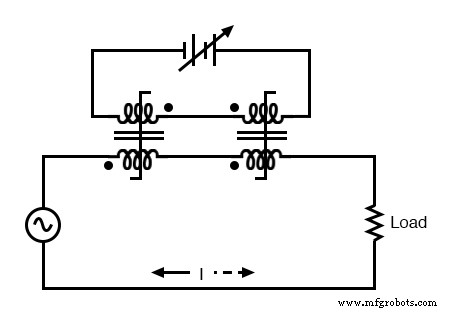
Out of phase DC control windings allow symmetrical control of AC.

Notice the placement of the phasing dots on the two reactors:the power windings are “in phase” while the control windings are “out of phase.” If both reactors are identical, any voltage induced in the control windings by load current through the power windings will cancel out to zero at the battery terminals, thus eliminating the first problem mentioned.

Furthermore, since the DC control current through both reactors produces magnetic fluxes in different directions through the reactor cores, one reactor will saturate more in one cycle of the AC power while the other reactor will saturate more in the other, thus equalizing the control action through each half-cycle so that the AC power is “throttled” symmetrically.

This phasing of control windings can be accomplished with two separate reactors as shown, or in a single reactor design with intelligent layout of the windings and core.

Saturable reactor technology has even been miniaturized to the circuit-board level in compact packages more generally known as magnetic amplifiers .

I personally find this to be fascinating:the effect of amplification (one electrical signal controlling another), normally requiring the use of physically fragile vacuum tubes or electrically “fragile” semiconductor devices, can be realized in a device both physically and electrically rugged.

Magnetic amplifiers do have disadvantages over their more fragile counterparts, namely size, weight, nonlinearity, and bandwidth (frequency response), but their utter simplicity still commands a certain degree of appreciation, if not practical application.

Saturable-core reactors are less commonly known as “saturable-core inductors” or transductors .

Scott-T Transformer

Nikola Tesla’s original polyphase power system was based on simple to build 2-phase components. However, as transmission distances increased, the more transmission line efficient 3-phase system became more prominent. Both 2-φ and 3-φ components coexisted for a number of years.

The Scott-T transformer connection allowed 2-φ and 3-φ components like motors and alternators to be interconnected. Yamamoto and Yamaguchi:

In 1896, General Electric built a 35.5 km (22 mi) three-phase transmission line operated at 11 kV to transmit power to Buffalo, New York, from the Niagara Falls Project. The two-phase generated power was changed to three-phase by the use of Scott-T transformations.

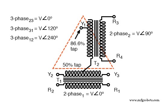
Scott-T transformer converts 2-φ to 3-φ, or vice versa.

The Scott-T transformer set, Figure above, consists of a center tapped transformer T1 and an 86.6% tapped transformer T2 on the 3-φ side of the circuit. The primaries of both transformers are connected to the 2-φ voltages.

One end of the T2 86.6% secondary winding is a 3-φ output, the other end is connected to the T1 secondary center tap. Both ends of the T1 secondary are the other two 3-φ connections.

Application of 2-φ Niagara generator power produced a 3-φ output for the more efficient 3-φ transmission line. More common these days is the application of 3-φ power to produce a 2-φ output for driving an old 2-φ motor.

In the Figure below, we use vectors in both polar and complex notation to prove that the Scott-T converts a pair of 2-φ voltages to 3-φ. First, one of the 3-φ voltages is identical to a 2-φ voltage due to the 1:1 transformer T1 ratio, VP12=V2P1.

The T1 center tapped secondary produces opposite polarities of 0.5V2P1 on the secondary ends.

This ∠0° is vectorially subtracted from T2 secondary voltage due to the KVL equations V31, V23.

The T2 secondary voltage is 0.866V2P2 due to the 86.6% tap. Keep in mind that this 2nd phase of the 2-φ is ∠90°. This 0.866V2P2 is added at V31, subtracted at V23 in the KVL equations.

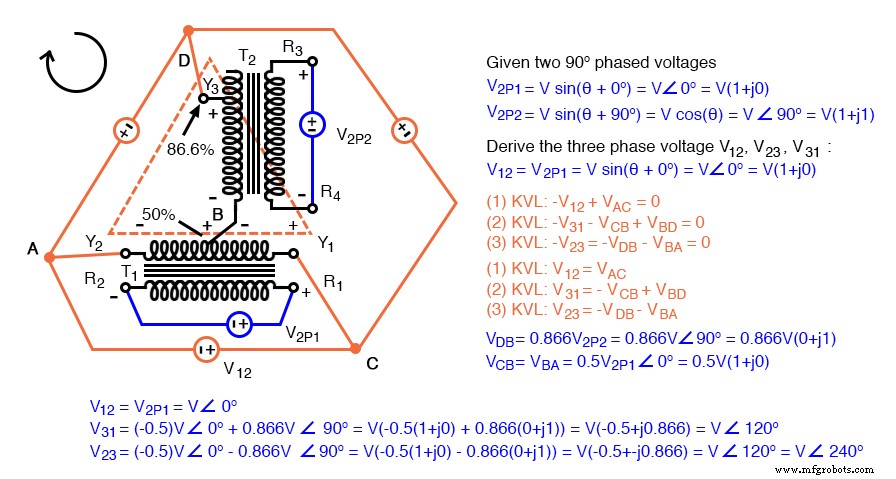
Scott-T transformer 2-φ to 3-φ conversion equations.

We show “DC” polarities all over this AC only circuit, to keep track of the Kirchhoff voltage loop polarities. Subtracting ∠0° is equivalent to adding ∠180°. The bottom line is when we add 86.6% of ∠90° to 50% of ∠180°we get ∠120°. Subtracting 86.6% of ∠90° from 50% of ∠180° yields ∠-120° or ∠240°.

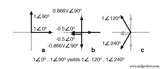
Graphical explanation of equations in Figure previous.

In Figure above we graphically show the 2-φ vectors at (a). At (b) the vectors are scaled by transformers T1 and T2 to 0.5 and 0.866 respectively. At (c) 1∠120° =-0.5∠0° + 0.866∠90°, and 1∠240° =-0.5∠0° - 0.866∠90°. The three output phases are 1∠120° and 1∠240° from (c), along with input 1∠0° (a).

Linear Variable Differential Transformer

A linear variable differential transformer (LVDT) has an AC driven primary wound between two secondaries on a cylindrical air core form (figure below). A movable ferromagnetic slug converts the displacement to a variable voltage by changing the coupling between the driven primary and secondary windings.

The LVDT is a displacement or distance measuring transducer. Units are available for measuring displacement over a distance of a fraction of a millimeter to a half a meter. LVDT’s are rugged and dirt resistant compared to linear optical encoders.

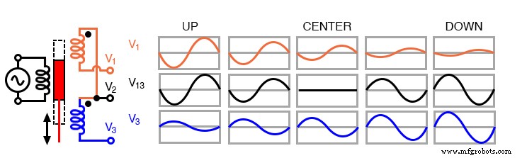
LVDT:linear variable differential transformer.

The excitation voltage is in the range of 0.5 to 10 VAC at a frequency of 1 to 200 Khz. A ferrite core is suitable at these frequencies. It is extended outside the body by an non-magnetic rod. As the core is moved toward the top winding, the voltage across this coil increases due to increased coupling, while the voltage on the bottom coil decreases.

If the core is moved toward the bottom winding, the voltage on this coil increases as the voltage decreases across the top coil. Theoretically, a centered slug yields equal voltages across both coils. In practice leakage inductance prevents the null from dropping all the way to 0 V.

With a centered slug, the series-opposing wired secondaries cancel yielding V13 =0. Moving the slug up increases V13. Note that it is in-phase with with V1, the top winding, and 180° out of phase with V3, bottom winding.

Moving the slug down from the center position increases V13. However, it is 180° out of phase with with V1, the top winding, and in-phase with V3, bottom winding. Moving the slug from top to bottom shows a minimum at the center point, with a 180° phase reversal in passing the center.

评论：

• Transformers can be used to transform impedance as well as voltage and current. When this is done to improve power transfer to a load, it is called impedance matching .
• A Potential Transformer (PT) is a special instrument transformer designed to provide a precise voltage step-down ratio for voltmeters measuring high power system voltages.
• A Current Transformer (CT) is another special instrument transformer designed to step down the current through a power line to a safe level for an ammeter to measure.
• An air-core transformer is one lacking a ferromagnetic core.
• A Tesla Coil is a resonant, air-core, step-up transformer designed to produce very high AC voltages at high frequency.
• A saturable reactor is a special type of inductor, the inductance of which can be controlled by the DC current through a second winding around the same core. With enough DC current, the magnetic core can be saturated, decreasing the inductance of the power winding in a controlled fashion.
• A Scott-T transformer converts 3-φ power to 2-φ power and vice versa.
• A linear variable differential transformer , also known as an LVDT, is a distance measuring device. It has a movable ferromagnetic core to vary the coupling between the excited primary and a pair of secondaries.

相关工作表：

• AC Metrology Worksheet
• Impedance Matching With Transformers Worksheet