来自纳米级脂肪分形的小角度散射

介绍

许多在纳米和微米尺度上生成的层次结构具有几何特征，这些特征在尺度膨胀下是不变的，表现出自相似性，因此具有分形特性 [1, 2]。尽管材料科学和纳米技术的最新进展允许制备具有精确自相似性的各种人工纳米/微米级确定性分形 [3-7]，但绝大多数自然过程会产生随机的、统计上的自相似性分形。在自然分形地层的结构研究中，可以借助确定性分形模型进行很好的近似，其分形维数与随机分形维数相同。这种方法已成功用于表明随机分形表面上的转移非常接近确定性模型几何结构的响应 [8]。通过在确定性分形的构造算法中引入多分散性，可以获得与对应于随机分形的那些类似的小角散射 (SAS) 强度 [9]。此外，“确定性”方法在计算上更有效，允许对分形形式、结构因素和回转半径等各种属性进行分析描述。

确定确定性分形和随机分形 [10, 11] 的结构特性的最可靠方法之一是在纳米或微结构材料上小角度散射的背景下使用波衍射，使用中子或电磁波 (x -射线、光等）[12]。这就是为什么，与该研究领域的实验确定相关的理论描述的基本任务之一是揭示分形结构与其对应的衍射光谱或散射强度分布与散射波矢量之间的关系。在这个方向上进行了大量的实验和理论研究[13-21]。

使用标准理论计算和插值，从这些实验测量中确定的参数是质量分形维数 D m（见附录 1），带有 D mD s，与 d −1<D s<d .我们用 d 表示 嵌入分形的欧几里得维度。质量分形维数描述了质量 M (r ) 在嵌入半径为 r 的圆盘中时会发生变化 .获得的质量半径 关系 \(M(r) \propto r^{D_{\mathrm {m}}}\) 导致散射强度的行为 \(I(q) \propto q^{-D_{\mathrm {m} }}\）。显然，D m 可以用散射强度的幂律相关性的指数确定为散射波矢量 q 的函数 [18, 22]。 D 的值越高 m，结构越紧凑。类似地，在表面分形的情况下，其表面分布服从 \(S(r) \propto r^{2-D_{\mathrm {s}}}\)，因此，\(\phantom {\dot { i}\!}I(q) \propto q^{-(2\mathrm {d}-D_{\mathrm {s}})}\) [19, 23]。在三维欧几里得空间中工作，D 当表面几乎完全光滑时，s 接近最小值 2。如果折叠得几乎完全填满空间，则它趋向于最多三个。

来自各种化学合成和生物系统的许多实验衍射强度在双对数标度上以连续的幂律衰减为特征，由恒定强度的区域交错。对于某些聚合物凝胶 [24]、用于纤维二糖底物的糖苷水解酶 [25]、聚电解质复合凝聚层 [26] 或纳米多孔碳 [27]，可以确定这种行为。尽管经典 Beaucage 模型 [28] 可以提供有关这些系统的基本结构信息（即质量或表面分形维数以及每个结构级别的总体尺寸），但由于对应于分形维数的固定值。 Cherny 等人最近部分解决了这个问题。 [29] 在小角度散射 (SAS) 模型的背景下。结果表明，对于具有单一尺度的确定性质量分形，可以获得额外的信息，例如分形迭代次数、基本组成单元的数量和比例因子。如果散射分布中存在连续的幂律衰减，则该方法还成功地用于开发脂肪分形的新模型。它可以应用于基本组成单元的整体尺寸与它们之间的距离在同一数量级的结构[30, 31]。

本文提出的理论模型结合了以前的模型以扩展其适用性。它描述了幂律衰减的连续性，散射指数的值任意减小，和 由恒定强度的区域交错。我们的模型还能够提供有关纳米/微米分形中每个结构级别的更详细信息。为此，我们考虑一个胖分形，由二维确定性质量分形表示，其缩放因子取决于迭代次数，但在大量迭代的限制内具有非消失表面积，因此具有正勒贝格度量。我们推导出了分形形式和结构因子的解析表达式，并展示了如何确定每个结构级别的分形维数和比例因子。

理论背景

考虑一组定向相似、相同的衍射孔径，这里用 Σ 表示 , 包含 N 透明区域，标记为 j ，必须考虑从每个孔径获得的幅度的总和。因此，众所周知的单个孔径衍射幅度的频率分布（附录2中的方程（37））可以改写为[32]：

j 局部坐标系中点的坐标 第一个光圈是 (x j ,y j ) 和 T (x,y ) 表示每个透明区域对应的单个传输函数。可以用积分交换求和，因为在我们的例子中，孔径是由相同的个体分布函数描述的，所以等式。 (1) 可以改写为：

来自前面等式的积分因子代表每个相同孔径的分布函数的傅立叶变换，如上所述。该幅度由包含求和的因子调制，表示形式为 \(A_{\delta }~=~\sum _{j~=~1}^{N}(x~ -~x_{j})(y~-~y_{j})\)。因此，阵列内部孔径的空间分布也被考虑在内。因此，方程。 (2) 可以改写为数组定理[32]的形式：

衍射图像在傅立叶平面内的强度分布变为：

正如预期的那样，乘积中的第一个因素对应于单个孔的散射强度，而第二个则揭示了这些孔在衍射孔径Σ内的分布方式 .这些数量也称为形状因子 F (p,q ) 和结构因子 S (p,q ）。这就是为什么，整篇论文中获得的结果将使用以下散射强度形式表示：

胖分形模型和方法

构建细（规则）康托分形的详细过程是众所周知的 [33]。这里只总结了主要的构建过程。采用自上而下的方法。从边 l 的初始正方形（或任何其他欧几里得形状）开始 0 (在 m =0)，其中心与笛卡尔坐标系原点重合，边平行于坐标系轴，正方形内任意一点满足条件 −l 0/2≤x ≤l 0/2 和 -l 0/2≤y ≤l 0/2。在第一次迭代 (m =1)，正方形被分成其他四个正方形，边长为\(\beta _{\mathrm {s}}^{(1)}l_{0}\)。我们用 \(\beta _{\mathrm {s}}^{(1)} \equiv (1-\gamma _{1})/2\) 表示，其中 \(0 <\beta _{\mathrm { s}}^{(1)} <1/2\)，第一次迭代缩放因子，和 γ 1 在这一点上移除的长度的分数，如图 1 a, b) 对于 m =1. (⋯) 之间的数字，作为上索引出现，量化迭代次数。不得将其解释为幂函数的指数。在比例因子方面，四个正方形的位置由向量给出 \(\boldsymbol {a}_{j}~=~\left \{ \pm \beta _{\mathrm {t}}^{ (1)}l_{0}, \pm \beta _{\mathrm {t}}^{(1)}l_{0}\right \}\) 与所有可能的符号组合，其中 \(\beta _{ \mathrm {t}}^{(1)}~=~\left (1-\beta _{\mathrm {s}}^{(1)}\right)/2\) 用于进一步简化公式。由于数值计算的简单性，正方形被选为初始形状。可以考虑任何其他几何形状，例如圆形。选择其他形状的效果仅在形状因子的 Porod 区域观察到，超出了本文的范围。

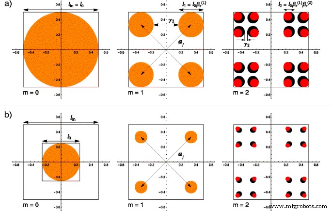
（在线颜色）前两次迭代的规则分形和胖分形的比较，其中 m 处的基本形状 =0 是直径 l 的圆盘 0 分形大小为 l 在：a l 0 =l 在; b l 0 =l 在/f , 与 f =2. 在这两种情况下，在 m =1 由于相等的缩放因子 \(\beta _{\mathrm {s}}^{(1)}\)，结构重合。以 m 开头 =2，胖分形有更大的比例因子\(\left (\beta _{\mathrm {s}}^{(2)}> \beta _{\mathrm {s}}^{(1)}\右)\)，因此，圆盘具有更大的直径（黑色圆盘 ) 而不是常规分形（红色圆盘 ); 一 j 是位置向量和 γ 我 是 i 处移除长度的分数 第一次迭代

上面描述的前两个步骤也应用于构造胖分形的经典版本，迭代 m =0 和 m =1. 这就是为什么，到目前为止，这两种结构是一致的。为了获得胖分形，对迭代 m 中使用的算法进行了修改 =1 必须通过在 m 处选择另一个缩放因子来完成 =2, \(\beta _{\mathrm {s}}^{(2)} \equiv (1 - \gamma _{2})/2\)。在高迭代次数的限制下应用整个算法 [34, 35]，重新获得胖分形的经典版本。从构造中可以清楚地看出，当每次迭代中的缩放因子选择为相等 \(\beta _{\mathrm {s}}^{(1)}~=~ \beta _{\mathrm {s}}^{(2)}~=~\cdots =\beta _{\mathrm {s}}^{(m)}\).

为了在 SAS 强度的行为中获得两个幂律衰减之间的恒定平台，我们必须考虑到散射单元之间的距离远大于它们的整体尺寸。这种方法首先用于表面分形模型 [36, 37]。考虑比率 f 散射单元之间的总距离l in 和它们的整体尺寸 l 0，一个有：

对于在两个分形区域之间显示恒定强度平台的散射实验，f 的值 ≫ 1 应该被选择。在表面分形的情况下，增加 f 的值 一方面使总 SAS 强度与独立散射单元的近似值之间具有更好的一致性 [36, 37]。

使用上述考虑，可以描述常规分形和胖分形之间的差异。 f因素的影响 ，上面介绍的，也可以可视化。这就是为什么在图 1 中，我们使用半径为 r 的圆盘以图形方式举例说明了比较 0≡l 0/2=l 在/(2f ) 作为我们的基本形状。前两次迭代的结果显示在图 1 的每一行中，表示为规则分形（用红色圆盘标记）和胖分形（用黑色圆盘表示）获得的结构，它们也可以完全重叠（标记为橙色磁盘）。在标记为图 1a 的行中，因子 f 被认为等于单位，从而获得经典结构和分形形状。该图的第二行，表示为图 1b，显示了上述因素的影响。在这些计算中，我们选择了 f 的任意值 =2. 观察到在迭代 m =0 和 m =1，在a和b两种情况下，得到的正则康托集和胖康托集的结构完全相同，完全重叠。由于共同的比例因子，这是可以预料的。然而，从图 1 的最后一对图像中可以看出，从 m 开始 =2，胖分形的圆盘半径更大，因为根据定义，它的比例因子 \(\beta _{\mathrm {s}}^{(2)}\) 大于常规的比例因子。在图 2b 的最后一张图像中，由于 f 因子的非单一值，圆盘的大小比图 2a 中的圆盘小得多 .

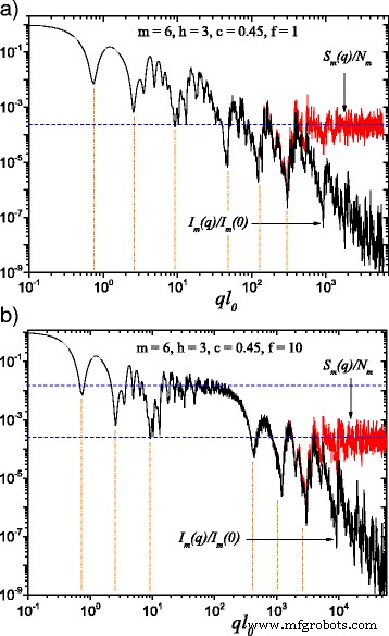
（在线颜色）方程给出的散射强度之间的比较。 (22) (黑色曲线 ) 和等式给出的结构因子。 (24) (红色曲线 ) 在 m =6 并根据等式在方向上取平均值。 (25)。在这里，h =3（即，缩放因子在三个连续迭代中保持不变），而计算散射强度的基本形状是边缘尺寸 l 的平方 0：a l 0 =l 在; b l 0 =l 在/f （与 f =10）。当 f ≠1，在两个广义幂律衰减之间出现恒定强度的平台（图 2 b）。 水平线 表示结构因子的渐近线 ≃1/N 米 ，而最小值位置是根据等式估计的。 (26)

为了获得幂律本身，需要进一步推广经典的脂肪分形模型。这是通过考虑缩放因子的变化不是在每次迭代中完成的，而是每隔一秒、三次、⋯，或者一般来说，每 h 第 次迭代。 m 处去除长度的分数 第一次迭代是：

与 0<c <1.函数 p 米 定义为：

对于 m 的任何正整数值 , 与 h =1,⋯,m ，其中使用了楼层函数 ⌊⋯ ⌋。因此，对应于 m 的缩放因子 第 次迭代由下式给出：

现在很清楚函数 p 的目的 米 是保持 h 的比例因子不变 迭代 (h <米 ).

每个正方形的位置向量的分量可以写成：

而每个正方形的边长由下式给出：

因子 f 用于长度l的公式 0 以考虑 (h +1)th 和 m th，正方形的大小随着它们之间的距离减小：

其中 h <米 .每次迭代的方格数为：

因此，在每个尺度上，被视为具有恒定缩放因子的迭代，一个具有由 [29, 38, 39] 给出的不同分形维数：

在大量迭代的限制下，构建的分形集的分形维数将为[34]：

这是二维脂肪分形的期望值。最后，如果 a 我 是在 i 处移除的相对面积 第 次迭代，则 \(\prod _{i=1}^{m}(1-a_{i})> 0\) 如果 \(\sum _{i=1}^{\infty } a_{i} <\infty \)，因此该模型满足胖分形的定义和特征[35]。

结果与讨论

根据巴比涅原理，我们可以得出结论，在 m 第 t 次迭代，光栅中的孔径是分形中剩余的正方形，而被去除的部分对辐射变得不透明。

单分散散射强度和结构因子

为了推导出胖康托分形散射强度的解析表达式，我们首先写出对应于 1D 的任意迭代的光栅透射率的递推关系 案件。 米 =0，我们有

考虑到分形的构造算法，第一次迭代后的透射率由下式给出：

$$ \begin{aligned} T_{1}(l_{1}, x,) =T_{0}(l_{1}, x) \ast \delta\left(\frac{x-l_{0}\ beta_{\mathrm{t}}^{(1)}}{l_{1}}\right) + \\ T_{0}(l_{1}, x) \ast \delta\left(\frac{x +l_{0}\beta_{\mathrm{t}}^{(1)}}{l_{1}}\right),~~~~~~~~~~~~ \end{aligned} $$ (17)

其中 δ (x -a ) 是 x 处的一维 Dirac-delta 分布 =a .符号 * 代表卷积算子。因此，在 m 第 t 次迭代，我们可以写成：

$$ \begin{aligned} T_{m}(l_{m}, x) =T_{m-1}(l_{m}, x) \ast \delta\left(\frac{x-u_{m} {l_{m}} \right) + \\ T_{m-1}(l_{m}, x, y) \ast \delta\left(\frac{x+u_{m}}{l_{m }} \right),~~~~~~~~~~~~ \end{aligned} $$ (18)

其中 \(u_{m}~=~l_{0}\beta _{\mathrm {t}}^{(m)}\prod _{j=1}^{m-1}\beta _{\mathrm {s}}^{(j)}\)。对等式执行傅里叶变换。 (18) 发现 m 处的散射幅度 第一次迭代是：

$$ A_{m}(p)=2^{m}\frac{\sin(\pi p l_{m})}{\pi p l_{m}}\prod\limits_{i=1}^{ m}\cos(2\pi p u_{i})。 $$ (19)

由于 2D 脂肪分形模型是两个一维脂肪分形的直积，其傅里叶变换可以写成两个一维傅里叶变换的乘积。因此，二维散射幅度可以写为：

$$ A_{m}(p,s)\equiv A_{m}(p) A_{m}(s), $$ (20)

因此，

$$ \begin{aligned} A_{m}(p, s) =N_{m}\frac{\sin(\pi p l_{m})}{\pi p l_{m}}\frac{\sin (\pi s l_{m})}{\pi s l_{m}} \times \\ \prod\limits_{i=1}^{m}\cos(2\pi p u_{i})\cos (2\pi s u_{i}), \end{aligned} $$ (21)

使散射强度变为：

$$ \begin{aligned} I_{m}(p, s) =\left(\frac{\sin(\pi p l_{m})}{\pi p l_{m}}\frac{\sin( \pi s l_{m})}{\pi s l_{m}} \right)^{2} \times \\ N_{m}^{2} \left(\prod\limits_{i=1}^ {m}\cos(2\pi p u_{i})\cos(2\pi s u_{i}) \right)^{2}。 \end{对齐} $$ (22)

前面方程中的第一个因子，表示由于形状因子引起的衍射强度，如方程 1 中所述。 (5)：

$$ F_{m}(p, s) =\left(\frac{\sin(\pi p l_{m})}{\pi p l_{m}}\frac{\sin(\pi s l_{ m})}{\pi s l_{m}} \right)^{2}, $$ (23)

对应于从边缘 l 的单个正方形获得的散射强度 米 .第二个因素，代表由于结构因素引起的衍射强度，如方程 1 中所述。 (5)：

$$ S_{m}(p, s) =N_{m}^{2}\left(\prod\limits_{i=1}^{m}\cos(2\pi p u_{i})\cos (2\pi s u_{i}) \right)^{2}, $$ (24)

描述了正方形的分布方式。总散射辐射强度是F的乘积 米 (p,s ) 和 S 米 (p,s ).

强度的幂律衰减，如公式 1 所示。 (22)，是在对所有方向进行平均后获得的 [29]。考虑到任何方向的概率相等，在二维分形的情况下，可以通过对散射矢量 q 的所有方向进行积分来计算平均值 =(p,s ）：

$$ \langle f(p, s) \rangle =\frac{1}{2\pi} \int_{0}^{2\pi}f(q,\phi)\mathrm{d}\phi, $ $ (25)

其中 p =q cosφ 和 s =q sinϕ .因此，散射强度I (q ) 作为动量传递模量的函数获得 q ≡|q |.

因为，从结构因子的定义来看，有\(S_{m}(0)~=~N_{m}^{2}\)，其中N 米 是正方形的数量，如等式中所定义。 (13)、标准化S的标准程序 米 可以采用(0) =1，如[11, 29]所述。

单分散散射强度I的计算结果 米 (q ) 和结构因子 S 米 (q ), 与 m =6，对于经典的脂肪分形（f =1 在图 2 a) 中，对于在这项工作中开发的扩展脂肪分形模型 (f =图 2b) 中的 10。为了获得图 2b，我们考虑了 h =3 以便前三个迭代的缩放因子 \(\beta _{\mathrm {s}}^{(1)}\) 保持不变，然后它有另一个常数值 \(\beta _{\ mathrm {s}}^{(2)}\) 用于接下来的三个迭代。正如预期的那样，在这两种情况下（对于 f =1 和 f =10)，一方面是散射强度，另一方面是结构因子之间的差异，当\(q \gtrsim 1/l_{m}\) 时可以观察到。在该区域，散射强度呈幂律衰减I (q )∝q ⁻³ .结构因子具有趋于 1/N 的渐近值 米 ，由图2a中的水平线或图2b中下方的水平线表示[29, 33]。

可以在图 2a 中看到连续两个广义幂律衰减，可识别为最大值和最小值在简单幂律衰减上的叠加。但在图 2b 中，强度近似恒定的区域，在域 20≲ql 0≲100，可以清楚地区分，包含在两个连续的广义幂律衰减中。这是由于正方形的大小减少了一个数量级 (f =10) 与它们之间的距离相比。这个区域，可以在图 2b 的上水平线周围观察到，具有渐近线 1/N 3，与经典胖分形的结构因子之一相同，表现出与仅考虑前3次迭代的情况相似的行为。

此外，从图 2 中可以看出，每个尺度的最小值的数量与恒定缩放因子迭代的数量一致。当穿过分形内不同方块的辐射发生干涉并且相位相反时，就会出现这些最小值，因此，方块中心之间最常遇到的距离 (2u 米 ) 等于 π /q .这就是为什么，最小值的近似位置是从关系中获得的：

$$ q_{i} \simeq \frac{\pi}{2 u_{i}},~~~~i=1, \cdots, m $$ (26)

在图2中由垂直线表示。对于前六次迭代，观察到使用方程计算的位置之间非常一致。 (26) 以及那些在散射强度或结构因子中发现的。这种近似对于更高的迭代可能不太准确，一旦迭代次数增加到某个值以上，因为在这些情况下，越来越多的距离与最常遇到的距离相当。尽管如此，这种近似在实践中应该会很好地工作，人们很难期望区分超过四个或五个这样的最小值。

对于每个单独的尺度，在给定的范围内 1/(2u 我 )≲q ≲1/(2u 我 +1)，衍射图案是由仅 i 的干涉产生的 分形迭代。这可以用来表明，在这个区间内，函数 I 米 (q )q ^D 和 S 米 (q )q ^D 是对数周期 [29]，其中 D 是对应于给定尺度的分形维数。特别是，对于图 1 和 5 所示的结果。 2和3，函数I 米 (q )q ^-1.1 和 S 米 (q )q ^-1.1 对于前三个迭代，周期为 \(1/\beta _{\mathrm {s}}^{(1)}\) 的对数周期，而 I 米 (q )q ^−1.51 和 S 米 (q )q ^−1.51 对于第二组三个迭代，是对数周期的，\(1/\beta _{\mathrm {s}}^{(2)}\)。

<图片>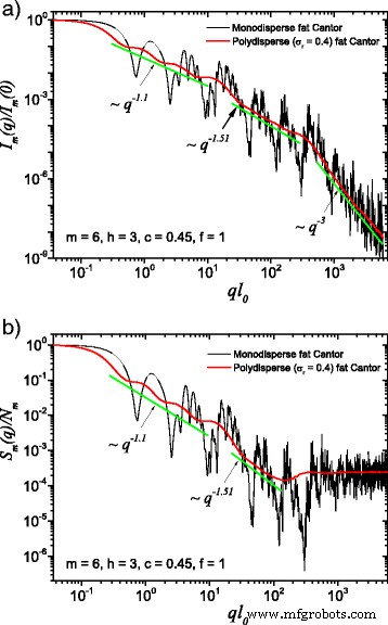

（在线颜色）单分散和多分散系统之间的比较：a 散射强度（方程（22））； b 结构因子（方程（24）），在分形的所有方向上取平均值，根据方程。 (25)。在这里，f =1, 米 =6, h =3（即缩放因子在连续三次迭代中保持不变），基本形状为初始边长l的正方形 0 =l in. 对于这两种情况，多分散性抹掉了单分散性的散射曲线，分形维数可以在每个结构层次上恢复

以与确定性质量分形类似的方式，方程。 (26) 可用于获得表征脂肪分形的几个结构参数。首先，最小值的总数与分形迭代的总数一致。图 2 显示分形由三个缩放因子为 \(\beta _{\mathrm {s}}^{(1)}\) 的迭代和三个缩放因子为 \(\beta _{\mathrm {s} }^{(2)}\)。其次，从这些最小值的周期性（或从 I 米 (q )q ^D 和 S 米 (q )q ^D )，缩放因子可以恢复。在图 2b 中，缩放因子 \(\beta _{\mathrm {s}}^{(1)}\) 可以从 ql 处的最小值的周期性获得 0≃7,25 和 90，而缩放因子 \(\beta _{\mathrm {s}}^{(2)}\) 可以从 ql 处的最小值的周期性中获得 0≃400,1000 和 2500。此外，分形区域之间的中间平台的长度可以用作比值 (f ) 的散射单元之间的距离，以及它们的整体大小。在图2b中，这个范围对应于13≲ql 0≲130。

多分散散射强度和结构因子

在我们工作的这部分中，我们现在可以考虑光栅尺寸服从分布函数 D N(l 0)，以这样的方式定义 D N(l 0)dl 0 给出分形光栅尺寸在区间 (l 0,l 0+dl 0）。这一步在我们的脂肪分形模型中引入了多分散性。我们通过选择对数正态分布来举例说明：

$$ D_{\mathrm{N}}(l_{0}) =\frac{1}{\sigma l_{0} (2\pi)^{1/2}}e^{-\frac{\left (\log(l_{0}/\mu)+\sigma^{2}/2\right)^{2}}{2\sigma^{2}}}, $$ (27)

相对方差 \(\sigma _{\mathrm {r}} =\left (\left \langle l_{0}^{2} \right \rangle _{D} - \mu ^{2}\right)^ {1/2}/\mu \)，平均值μ =<l 0〉 D , 和方差 \(\sigma =\left (\log \left (1+\sigma _{\mathrm {r}}^{2}\right)\right)^{1/2}\)。使用方程(21)和(27)得到分布函数上平均的多分散强度：

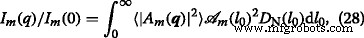
在哪里 is the corresponding area at m 第 次迭代。 The structure factor is calculated in a similar manner, but without the term [29].

The computed results in the case of polydisperse (red curves) and monodisperse (black curves) scattering intensities (labeled by a) and structure factors (labeled by b) can be seen in Figs. 3 and 4. The difference between them is given by the value of the f 因素。 In Fig. 3, the classical construction of a fat fractal was used so that f =1, while taking into account the smaller sizes of the basic units leads to the choice of f =10 in Fig. 4. Polydispersity is calculated for a relative variance of σ r =0.4. It can be seen that the oscillations are smeared out, the overall amplitude decreases, so that the scattering curves become smoother [29, 40]. However, for this particular value of σ r, the positions of main minima and maxima are still observable.

(Color online) A comparison between monodisperse and polydisperse systems:a scattering intensity (Eq. (22)); b structure factor (Eq. (24)), averaged over all orientations of the fractal, according to Eq. (25)。 Here, f =10 (and thus, a region of constant intensity appears at about 20≲ql 0≲100), m =6, h =3 (i.e., the scaling factor is kept constant for three consecutive iterations), and the basic shape is a square of initial edge length l 0 =l in. For both cases, the polydispersity smears out monodisperse scattering curves, and the fractal dimensions can be recovered at each structural level

More generally, for small values of σ r (i.e., small enough that the oscillations are observable), the estimation given by Eq. (26) can be still used. Hence, the number of fractal iterations, the scaling factor at each structural level, the ratio of the distances between scattering units, and their overall size can be recovered. When σ r is increased to high enough values so that oscillations are completely smeared out, the scattering curves become simple power-law decays. Since we used a narrow bell-shaped distribution, the scattering exponent is preserved. Moreover, it gives, for each power-law decay, the fractal dimension of that particular structural level. This is in good agreement with the theoretical estimation of Eq. (14). This is also in accordance with experimental setups, where almost every scattering curve has a certain degree of polydispersity. Thus, our developed fat fractal model, with an interleaved region of constant intensity, recovers the fractal dimension at each structural level from polydisperse experimental data.

结论

In this article, we suggest a theoretical model that generalizes the standard one for nanoscale fat fractals. It is characterized by the fact that the initial edge size of the elementary unit shape is taken to be much smaller than that of the overall size of the fractal, and thus, much smaller than the distances between the elementary units inside the fractal. Figure 1 b illustrates the basic model, when a quotient of 1/2 is considered in-between these quantities, respectively.

Based on this model, an analytical formula is calculated and presented, in Eq. (22) for the scattering intensity and in Eq. (24) for the structure factor. Averaging over all possible orientations is done according to Eq. (25)。 These averaged quantities are characterized, on a double logarithmic scale, by the presence of two structural levels, and thus by two power-law decays interleaved by a region of constant intensity, represented by a plateau, as seen in Figs. 2 b and 4. This plateau coincides with the asymptotic region of the structure factor of the fat fractal, as if we would have considered only the contribution from the first structural level, when the scaling factor was kept constant. The asymptotic values of the plateaus can be used to obtain the number of scattering units for each structural level. The length of the plateau is controlled by the value of f . The power-law decays encompassing the plateau are obtained by keeping constant the scaling factors for a finite number of iterations, in our case, as an example, for three out of a total of six. The slope of the second power-law decay is higher because the values of scaling factors, by definition, increase at each structural level, and this is confirmed by our numerical computations, as can be seen in Figs. 2, 3, and 4.

We also described the polydisperse case of the fat fractal model. Here, the sizes of the composing units obey, as an example, a log-normal distribution function. We obtained smoothed curves for the scattering intensities and structure factors. The monodisperse scattering curves as well as the polydisperse ones, with small enough values of the relative variance, allow to obtain the scaling factors at each structural level, while the scattering exponents in the polydisperse curve give the fractal dimensions at each structural level. The chosen value of 0.4 for the relative variance is meant to illustrate the case in which one can still observe some minima in the scattering characteristics, and the curves still retain a shape close to power-law decays.

The results obtained in the framework of the suggested model can be used to reveal structural properties of fractal materials characterized by a regular law of changing of the fractal dimensions. The proposed model is also a very versatile one because it can be extended to include other features such as different shapes of the elementary unit, more than two structural levels, or it can be adapted to work in other Euclidean dimensions. These results are useful for a detailed description of experimental diffraction data in the context of small-angle scattering obtained from various complex nano- and micro- scaled hierarchical structures.

Appendix

fractal dimension

Mass and, respectively, surface fractal dimensions are probably the most important quantities that characterize a fractal. Actually, we will deal only with deterministic mass fractals, and we shall refer to mass fractal dimension, simply as the fractal dimension (D m).

In general terms, the mass-radius relation can be rewritten as [2]:

where the scaling law correction A (r ) tends to a constant value if r →∞ .

If it is known a priori that the structure is a fractal in the high number limit, the fractal dimension can be found straight from the first iteration. To illustrate this procedure, let us consider a fractal of size l 0, composed of k elementary units at the first iteration, each of size β s l 0, where β s is a scaling factor. Since the mass-radius relation, given by Eq. (29), is equivalent with the scale-invariance relation [2]:

one can write M (l 0)=kM (β s l 0）。使用方程。 (29), one obtains a direct method to compute the fractal dimension, via:

fraunhofer diffraction and the array theorem

Let us consider a two-dimensional diffracting aperture Σ , laid in the (x,y ) plane, illuminated in the positive z 方向。 In an observation plane (u,v ), parallel to Σ , the complex-valued amplitude of the obtained diffraction image, computed using the framework of scalar theory of diffraction, according to the Huygens-Fresnel principle, can be written as [41]:

In the previous formula, \(r =\sqrt {z^{2}+(u-x)^{2}+(v-y)^{2}}\) is the distance between two arbitrarily points taken, respectively, from the plane containing Σ and from the observation plane. For the Fraunhofer diffraction model to be applicable, this distance must satisfy the condition of being much bigger than the wavelength λ .

Performing a binomial expansion of the square root in Eq. (32) and retaining only the first two terms, one obtains [41]:

This approximation leads to the Fresnel diffraction integral:

where the prefactor P (u,v ) is given by

and k =2π /λ . Considering, in addition, that the condition z ≫k Max(x ² +y ² )/2 is satisfied, one has \(\text {Exp}{\left (\frac {k}{2z}(x^{2}+y^{2})\right)} \simeq 1\). Rewriting Eq. (34), the Fraunhofer approximation becomes:

Denoting the spatial frequencies with p =u /(λ z ) and s =v /(λ z ) and ignoring the multiplicative phase factor P (u,v ) preceding the integral in Eq. (36), the amplitude becomes simply the Fourier transform of the distribution of the Σ 光圈。 Considering that the illumination is made using a monochromatic, unit-amplitude plane-wave, at normal incidence, and that the field distribution across the aperture is equal to its transmission function T (x,y ), one obtains the frequency distribution of the diffraction amplitude in the phase space: