重新评估硅纳米晶体中的发光寿命分布

介绍

胶体纳米粒子可用于多种应用，包括催化、医疗和光电应用 [1,2,3,4]。半导体纳米粒子对光发射、光伏和光催化应用特别感兴趣 [5, 6]。由于硅的可调发射特性 [7] 以及硅的丰度和生物相容性 [8]，硅纳米晶体 (SiNCs) 是当前关注的焦点。为了开发基于纳米粒子的技术，需要深入了解相关的光电特性，而时间分辨光谱通常是实现此目的的宝贵工具。

SiNC 的发光寿命通常用拉伸指数 (SE) 函数建模，其基本形式为 exp[ - (λt ) ^β ]，其中色散参数β 取 0 到 1 之间的值，λ 是一个速率参数，t 是时候了。该函数通常被描述为“比指数慢”，并且暗示着衰减率的不对称分布向着更长的寿命方向发展。一旦 β 和 λ 通过拟合发光衰减曲线找到参数，可以近似重建相应的衰减率分布[9]。

在过去的 20 年里，硅和其他半导体量子点中 SE 发光衰减的起源引起了激烈的争论，而且争论最近还在继续 [10]。已经对衰减动力学中 SE 的出现提出了各种解释，包括载流子隧穿和捕获在紧密间隔的纳米晶体 [11]、不均匀加宽的尺寸分布 [12]、尺寸相关的电子-声子耦合 [10] ，以及非辐射复合的势垒高度分布 [13]，后者类似于先前对多孔硅的建议 [14]。显然，要更广泛地理解SiNCs以及半导体纳米晶体中的发光机制，需要了解速率分布。

在以前关于 SiNC 的许多文献中，拉伸指数衰减是先验假设的，通常没有分析其他可能的分布。 SE 倾向于在视觉上很好地拟合（即，最佳拟合线似乎与“肉眼”数据很好地匹配）。此外，在绝大多数以前的工作中，例如 [15]，对于是否实际模拟了种群衰减或发光衰减缺乏明确性。这些通过导数相关，应该使用正确的表达式来理解样本中的衰减时间尺度 [16]。此外，由于宽的集合发射光谱，探测器的响应度函数会对 SiNC 中测量的发光衰减曲线产生显着影响。尽管如此，响应度很少被考虑在内，因此很难比较不同调查的结果。最后，以前没有研究尝试在硅纳米晶体的分析中使用频率分辨光谱 (FRS)。原则上，FRS允许在不先验假设模型的情况下提取寿命分布。

本文的目的是建立一种方法来测量、模拟和解释硅纳米晶体的发光动力学。希望这有助于更好地理解文献中经常相互矛盾的结果的巨大多样性，导致不同测量之间更好的一致性或至少更高的一致性，并更好地理解发光机制。

基础理论

我们比较了三种模型：广泛用于 Si 纳米晶体的拉伸指数、最近首次应用于 SiNC 的对数正态衰减分布 [17] 和双分子衰减。对于任何模型，发射概率密度函数，用强度函数g的积分表示 (t )，在时间 t′ 与 t′ 处剩余的激发分数有关 根据[16]。

其中 c t 和 c 0 是 t 时刻被激发的 NC 的数量 和最初。概率密度函数描述了时间 0 和 t 之间发射的光子的分数 相对于发射的光子总数。如果种群衰减遵循一阶速率方程（即“单分子”重组），我们有 dc t /dt = − λc t , 其中 λ =1/τ 0 , 导致通常的 c t /c 0 =exp[− λt ] 和 g (t ) =λ⋅ exp[− λt ] 取等式两边的时间导数后。 1. 导数是必要的，因为在窗口dt'中测量的发光强度 与该区间内激发分数的变化成正比。

如果我们同时考虑辐射率和非辐射率，那么我们替换总衰减率 λ 与 λ R + λ NR 所以 g (t ) =(λ R + λ NR )exp[− (λ R + λ NR t ] =λ R exp[− (λ 里 + λ NR )t ] + λ NR exp[− (λ R + λ NR )t ] 其中只有第一项是可测量的，产生时间分辨光谱 (TRS) 的测量强度

用于拟合数据的衰减函数，I t =A· exp(− λt ) + dc，使用额外的任意前置因子 A 进行缩放 ，这取决于检测效率和激发的纳米粒子数量，并将导致适当的规模。通常在衰减函数中加入一个直流偏移作为另一个拟合参数。

在拉伸指数衰减的情况下，激发发射体的比例根据

其中 λ 东南 是拉伸指数衰减率（等于 1/τ 东南 ). 将其插入等式。 1 和前面一样取两边的导数得到一个发射概率函数为

一种估计频率分布的方法H (λ ) 导致方程。 3 使用拉普拉斯逆变换 [9] 显示，产生的分布随着 β 的减小而变宽 并且偏向高频。

不幸的是，在方程式中。 4、不可能将前因分为辐射和非辐射部分。这意味着方程。 4 仅针对 λ 正确归一化 NR = 0 [16]，从 PL 衰减曲线获得的寿命分布只能通过这种方式来理解。此外，前因子中有一个时间依赖项；因此，与发光衰减相比，种群衰减具有不同的时间依赖性 [16, 18]。为了获得τ的值 东南 和 β 对于可以从中提取适当平均寿命的种群衰减，必须使用等式。 4 模拟观察到的衰变，我们替换 g (t ) 由测量的衰减函数 I t :

在方程式中。 5、一个缩放参数（也可以吸收β 和 λ 前置因子中的项）和直流偏移作为拟合参数插入。平均寿命为

其中 Γ 表示 Gamma 函数，平均衰减时间为

在以前的许多工作中，通常使用“标准”拉伸指数 exp[− (λ 东南 t ) ^β ] 模拟发光衰减而不是种群衰减。因此，我们有一个归一化的强度函数由

等式 8 被归一化，使得 t 之间的积分 =0且∞等于1。对应的拟合模型很简单

等式 9 被广泛应用并且通常非常适合 SiNC 发光数据，尽管事实上（如等式 4）等式。对于 100% 的绝对量子效率 (AQY)，8 是严格归一化的。一个经常被忽视的一点是人们无法提取τ 东南 (=1/λ 东南 ) 和 β 从由方程建模的发光衰减。 9 并使用它们来计算方程的平均时间。 6 和 7。本质上，方程。图 4 和图 8 是不同的强度衰减模型，预计会有不同的种群衰减函数、平均时间和衰减率分布。

为了找到会导致由方程给出的强度函数的种群衰减。 9，我们应用我们从方程中得到的相同过程。 4 到等式。 5，但反过来，就是：

经过几个步骤，方程的解决方案。 10 是

方程 11 是从方程给出的强度衰减得到的种群衰减。 8. 以通常的方式求平均寿命导致

和平均衰减时间

最后，频率分布是 (1 /λ )·H (λ )，其中和以前一样，H (λ ) 是参考文献中计算的分布。 [9] 对于方程给出的种群衰减。 3. 这些结果总结在表1中。

两个 SE 公式之间的差异是显着的（图 1）。在文献中，人们经常发现强度衰减由A·建模 exp[− (t /τ 东南 ) ^β ] + dc（即方程 9），然后使用方程计算平均时间。 6 和 7。这在数学上似乎是不正确的，因为方程。图 6 和图 7 源自等式给出的强度衰减。 4，不等式。 8. 例如取τ 东南 =100 μs 和 β =0.7，如图 1 所示，对于由 exp[− (t /τ 东南 ) ^β ]，我们发现平均时间常数为 199 μs（方程 12），而使用方程为 127 μs。 6. 平均衰减时间也有类似的差异（方程 7 和 13）。此外，还有一种称为 Higashi-Kastner 方法的方法，用于估计特征寿命 [19]，该方法已应用于 SiNC，作为应用 SE 衰减模型的替代方法 [20, 21]。在该模型中，特征延迟时间 t d , 简单地将衰减数据的峰值绘制为 I t ·t 对比 t .这被建议等价于 (1 /β ) ^{1 /β} ·τ 东南 从方程获得。 9 [20]。

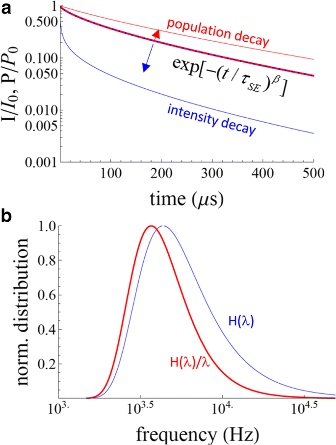
拉伸指数。 一 具有 τ 的拉伸指数函数的种群和强度衰减 东南 =100 μs 和 β =0.7。蓝红虚线为 exp[− (λt ) ^β ]。如果这代表人口衰减，那么强度衰减将由蓝线给出。如果 exp[− (λt ) ^β ] 是强度衰减，然后用红线显示种群衰减。 b 对应的速率分布

或者，衰减率的分布可以遵循特定的H (λ )，导致发光衰减：

其中 H (λ ) 表示衰减率的频率相关分布。等式 14 简化为等式。 2 如果 H (λ ) 等于狄拉克 delta 函数 δ (λ − λ 0)，或者它可以表示由所选分布加权的连续指数系列。对数正态函数在纳米晶体系统中似乎是一个合理的选择，因为许多纳米晶体集合自然地遵循对数正态尺寸分布 [22]。为了避免进一步的混淆，我们使用以下给出的对数正态函数的标准归一化定义：

所以测得的衰减函数为

与 SE 函数一样，只有两个独立变量（以及偏移量和比例因子）。时刻像往常一样定义；即，中间率由 exp 给出 (μ ), exp 的平均值 (μ + σ ² /2)，并且最可能的生命周期（分布的峰值）是 exp (μ − σ ² ）。以前，采用了非标准分布 [16]（即，虽然本身有效，但不是普遍接受的对数正态分布函数的分布）。公式 14 也适用于辐射衰减分布（即 AQY =100%）。事实上，有人建议衰减率分布由（未知）量子效率函数加权 [16]。在实际情况中，鉴于很难或不可能知道样本中非辐射率的总体分布，人们只能接受这一警告。

发光衰减也可能对应于二级反应（即“双分子”衰减）[23]。这里，人口衰减的速率由 dc 给出 /dt =− λ [c t ] ² , 产生剩余的分数 c t /c 0 =(c 0λt + 1) ⁻¹ .将此表达式插入等式。 1 导致幂律衰减：

双分子模型只有一个速率常数λ （与具有速率分布的拉伸指数和对数正态不同），并且没有平均寿命。更具体地说，时间积分发散，二阶衰减的平均寿命是无限的。

迄今为止，“标准”SE 函数（方程 9）一直是用于 SiNC 发光衰减的主要模型，许多论文致力于解释发光机制衰减的含义。对数正态寿命分布最近首次应用于 SiNC [17, 24, 25]。显然，假设任何模型都没有什么先验的理由，而是最好直接建立衰减率的分布。这至少在原则上可以通过正交频率分辨光谱（QFRS）来实现，该技术已多次应用于非晶硅，但未应用于 SiNC。

正交频率分辨光谱

QFRS 方法在文献中的报道相当少，主要限于对稀土掺杂玻璃的一些研究 [26,27 和 a-SiOx:H。 Mater Sci Eng B 105:165–168" href="/articles/10.1186/s11671-018-2785-x#ref-CR28" id="ref-link-section-d291096563e3613">28] 和非晶硅 [29, 30,31]. 该技术的基础是用角频率 ω 的正弦波调制泵浦光束激发样品 并在尝试跟踪激发时测量发光的相位和幅度。通过这种设置，正交分量 (Q ) 的相敏检测器（即锁定放大器）提供了寿命分布的直接测量 [30]。由于 AOM 调制激光振荡的幅度可以与频率相关，PL 的正交分量 Q PL =Z PL 罪 (Δθ PL ) 必须归一化为激光振荡的幅度，Z 洛杉矶 .

由于单个指数衰减不会导致 QFRS 频谱中的 delta 函数，因此正交 FRS 信号变得复杂。观察到的信号实际上是寿命分布与 [31] 在对数尺度上给出的单个指数响应函数的卷积。

其中时间常数τ 0 =ω 0 ⁻¹ .因此，除非衰减率分布在几十年范围内，否则必须执行反卷积以提取有意义的分布。

结果与讨论

基本特征

由于与 SiNC 相关的低对比度和来自无定形碳载体的重叠斑驳对比度，无法应用使用明场图像的基于计算机的粒子计数算法，并且必须使用像素计数软件“通过肉眼”估计直径（样品明场 TEM 图像如图 2a、d 所示，手动粒子计数结果与对数正态分布（图 2c、f）拟合，以获得 2.9 nm 的线性平均直径（平均值和标准偏差自然对数μ =1.057 和 σ =0.1555) 和 5.4 nm (μ =1.663 和 σ =0.1917)，分别为 1100 和 1200 °C 的退火温度。这些样品此后将被称为“小”和“大”SiNC。通过所选 NC 的高分辨率成像进一步检查尺寸（图 2b、e），其中晶格条纹可用作识别 NC 并估计其直径的另一种方式。傅里叶变换红外 (FTIR) 光谱和 XPS 数据表明制备的 SiNCs 成功地被十二烯官能化；然而，小SiNCs比大SiNCs氧化得更多，因此显示出较小的功能化程度（附加文件1：图S1和S2）。

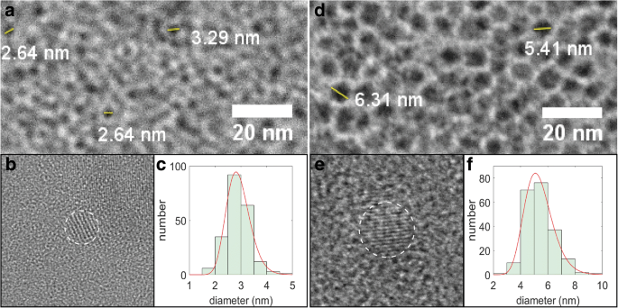
SiNC 的 TEM 图像。 一 明场，b 高分辨率和c 小 SiNC 的尺寸分布直方图。面板 d –f 表示来自大型 SiNC 的一组相似图像

光致发光和时间分辨光谱

光致发光 (PL) 光谱集中在 660 和 825 nm，小和大 SiNC 的半峰全宽分别为 123 和 198 nm（图 3 插图）。根据 \( {E}_g\kern0.5em =\kern0.5em \sqrt{E_{g,\mathrm{bulk}}^2\kern0.5em +\ kern0.5em D/{R}^2} \) [32] 与 D =4.8 eV ² /nm ² 和 R 是 NC 半径，这对于小颗粒非常一致，但预测的带隙比大颗粒的 PL 峰获得的带隙略小。小型 SiNC 样品的 AQY 为 12%，大型 NC 样品的 AQY 为 56%。两个样品在不同系统上的独立测量分别为 18% 和 48%，这是 AQY 测量 [33] 中不同激发波长和截止波长的典型不确定性。我们假设较大的 NC 的弯曲度较低、能量较低的表面导致更好的表面功能化，并且非辐射表面态对整个 PL 光谱的贡献较小。

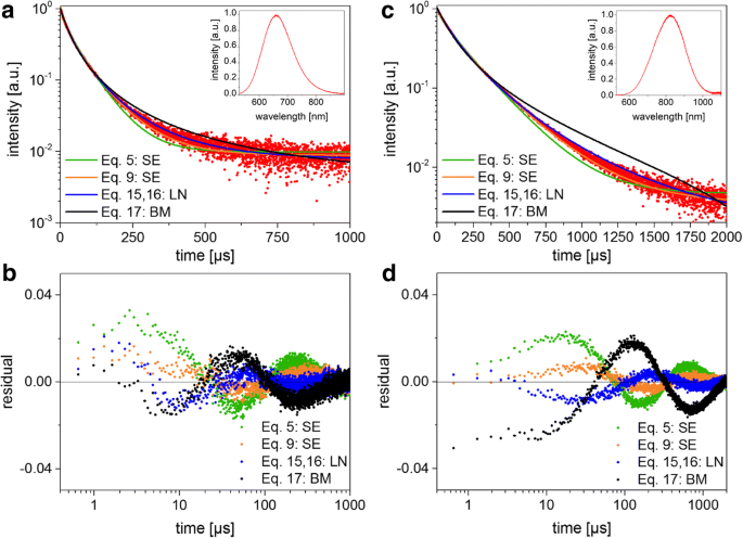
TRS 数据和拟合结果。 一 发光衰减和相应的拟合函数 (BM 双分子，SE 拉伸指数，LN 对数正态）用于小型 SiNC。 PL 光谱显示在插图中。 b (a 中拟合的残差图 , c , d ) 显示大 SiNC 的曲线和残差。

正如根据之前关于 SiNC 的广泛文献所预期的那样，两个样品都产生了非指数衰减。测量的 PL 衰减符合方程。 5、9、16 和 17，以便使用标准平方和最小化测试不同的模型（图 3）。稍后将讨论检测器响应度在宽 NC 发光光谱上不是恒定的事实。对于所有情况，残差都会波动，表明没有一个模型看起来完全足够，但“简单”SE 模型（方程 9）和对数正态模型（方程 16）倾向于残差平方和的最低值。两个 SiNC 样品的计算拟合参数和平均寿命如表 2 所示，其中的平均值显然取决于衰减模型的选择。还应用了 Higashi-Kastner 方法（图 4），并通过用倾斜的高斯拟合延迟时间曲线来确定峰值位置。 Higashi-Kastner 方法产生一个时间常数 t d 非常类似于 (1 /β ) ^{1 /β} ∙τ 东南 ，这些值取自等式。 9 如前文 [20] 所示。双分子模型拟合得相当差，与未严重过度激发的孤立纳米晶体一致。故不再赘述。

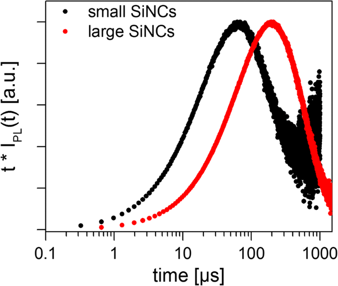
归一化 PL 衰减曲线乘以衰减时间（Higashi-Kastner 图），用于小型和大型 SiNC 系综。峰值位置代表最主要的衰减时间，用 t 表示 d 表2中

为了估计这些测量条件下每个 NC 的平均激子数量，必须从吸收截面计算激发率，显然可以高达 10 ^-14 厘米 ² 对于这些实验 [34]。假设激发辐照度为 4500 W/m ² 在 352 nm 和测量的峰值发射率（参见以下部分）下，估计大和小 SiNC 的每个 NC 的激发数分别小于 ~ 1 和 0.2。这表明大型 SiNC 可能略微过度兴奋。由于某些 NC 中存在多激子，这可能会导致额外的非辐射效应。为了进一步评估这种可能性，将寿命作为激发功率的函数进行测量；低至上述报告值的 2%。结果显示没有趋势，并且在 ~ 2% 内始终相同（附加文件 1 图 S3），尽管低功率测量中的信噪比较低，但仍接近拟合和可重复性误差。因此，NCs可能的过度激发似乎对结果影响不大。

为了估计来自 TRS 的寿命分布，使用具有 ~ 3 nm 带通的单色器在一组固定波长上测量衰减（图 5）。由于强度低，为此目的使用了光子计数 PMT 系统。对于有效的单色辐射，由于响应函数在如此窄的波长范围内的分布可以忽略不计，因此不同探测器测量的衰减常数应该没有差异。十二烷基封端的粒子也发现了与在其他硅 NC 中观察到的相同的趋势 [25, 35, 36]；也就是说，色散参数随着波长的变化而增加，并且寿命迅速增加（图 5，表 3）。

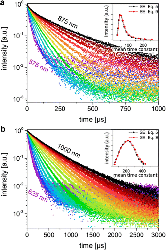
窄波长 PL 衰减。 一 在 575 到 875 nm 的特定发射波长 (3 nm FWHM) 下，小 SiNC 的发光衰减，间隔为 25 nm。数据符合方程。 5 和 9，这产生了几乎单一的指数拟合。 b 对于在相同条件下测量和拟合的大型 SiNC，发光在 625 到 1000 nm 的特定发射波长范围内衰减。表 1 中给出了小型和大型 SiNC 的时间常数

在相同的测量波长下，较小的颗粒总是比较大的颗粒具有更短的寿命。这一观察结果与较小粒子的较低 AQY 一致，表明大 NC 的寿命不太受非辐射过程的影响。与小 NC 样品相比，大 NC 的氧化程度也较低（附加文件 1 图 S1）。因此，虽然在小样品上观察到的较低 AQY 与测量的较短寿命一致，但不能通过波长选择对两个样品进行相对比较（基本上，发射波长取决于尺寸和 氧化程度[24]，这在两个样品中是不同的）。

还绘制为图 5 中的插图，是通过绘制从单色数据获得的平均寿命而获得的分布，使用方程。 5 或 9 以拟合数据，作为该波长处 PL 强度的函数。由于对于这些衰减，β 参数相当接近 1，因此使用两个版本的 SE 模型计算的平均寿命之间几乎没有差异，并且以这种方式获得的分布看起来很相似。由于对 I 的非辐射贡献，这些衰变并不代表寿命的“真实”分布 PL ，它们仍然可以给出寿命分布的指示。对于小颗粒，我们在 ~ 47 μs 处观察到一个峰值，而对于大 NC，峰值更对称，并以 220 μs 为中心。

频率分辨光谱

我们首先验证了来自两个测试标准的 FRS 数据：第一个是 RC 电路，第二个是荧光 Eu 螯合物掺杂微球 (Fisher Scientific) 的样本。 RC 电路具有单指数衰减，其中 FRS 数据与方程匹配。 9 非常接近并在 12.7 kHz 达到峰值，与测量的 78.9 μs 衰减时间常数一致。 Eu 螯合物 PL 光谱在 650 nm 处达到峰值，衰减时间约为数百微秒，为 Si NC 提供了标准。发光也几乎单指数衰减，寿命为 670 μs。 FRS 数据以~ 1570 Hz 为中心，宽度几乎等于响应函数（方程 18），这与观察到的 TRS 结果非常接近。差异（636 与 670 微秒）可能是由于与激发方法耦合的衰减的轻微非指数行为，如下文进一步讨论。

Si-NC 的 FRS 数据存在问题，因为观察到的 QFRS 结果仅比响应函数稍宽（参见图 6a 的插图）。因此，必须对数据执行去卷积，这些数据需要几乎没有噪声，以避免去卷积过程中出现重大问题。我们使用 Richardson-Lucy 反卷积方法 [37] 来强制执行正约束。去卷积和归一化 QFRS 数据然后直接产生测量的寿命分布，如图 6 所示，分别针对大和小 NC（红点），无需先验假设任何模型。对于这两个样本，我们发现了一个广泛的寿命分布，在大 NC 的情况下，稍微偏向更高的频率，而小 NC 分布在半对数图上更接近对称。小NC的衰减率分布在19,900 Hz (50.3 μs)处达到峰值，而对于较大的NC，衰减率分布在6280 Hz (159.2 μs)处达到峰值。

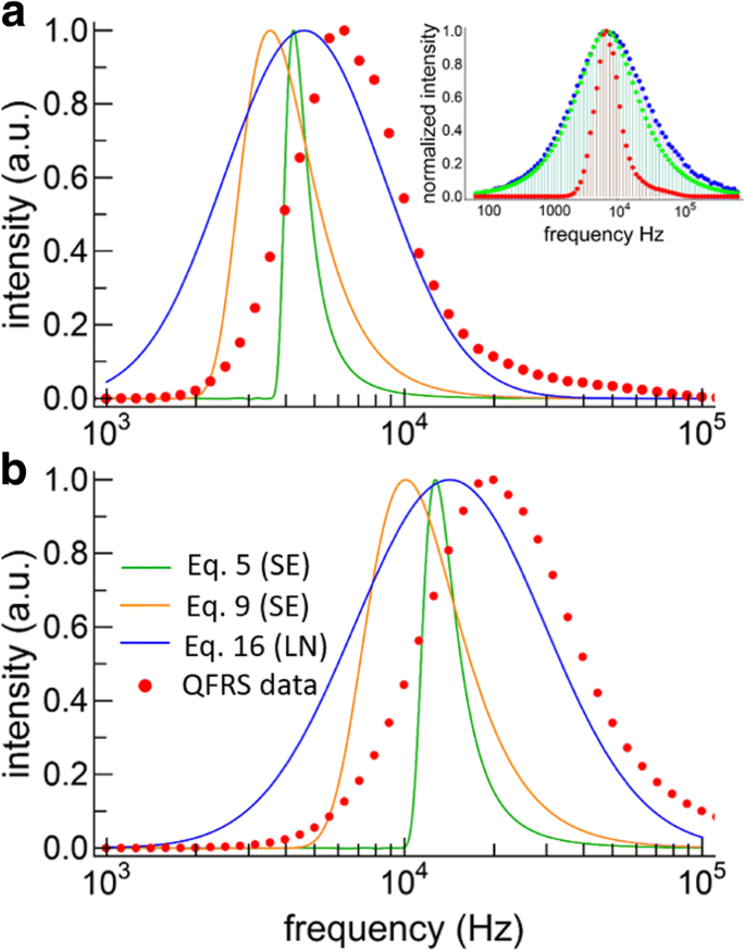
Lifetime distributions. 一 Lifetime distributions for large SiNCs obtained from fitting the TRS data with the two SE models and the LN model. The deconvolved QFRS data is also shown (red points). The inset shows the raw QFRS data for this sample (blue), the response function (green), and the deconvolution (red). b Lifetime distributions obtained by model fitting the TRS data (lines, same color scheme for both graphs) and QFRS (red points) for the small SiNCs

The lifetime distributions obtained from the stretched exponentials (orange and green curves) and lognormal (blue curve) model fits are also plotted in Fig. 6 for the large and small particles. The three decay models yield different distributions, both in terms of the overall shape and the peak frequencies. For both samples, the QFRS peaks at a higher frequency than any of the TRS model fits. While this may seem surprising, the same effects have been observed for CdSe NCs having a distribution of lifetimes [38, 39]. In fact, the TRS decay curve for CdSe NCs was evidently sensitive to the pulse duration, with shorter pulses accentuating the shorter lifetimes and the opposite case for long pulses. Furthermore, the mean lifetimes obtained by long-pulse duration techniques were a factor of 3–4 times longer than those obtained by phase measurement, which was due to preferential excitation of the long-lived population in steady-state excitation [38]. Indeed, the response function for TRS with a slow repetition rate is narrower than for FRS, cutting off especially sharply on the high frequency side [29]. Essentially, FRS accentuates the short-lived components of the ensemble decay more than steady-state TRS does, and this may account for the difference in the peak frequencies obtained by TRS model fitting and FRS. Despite these inherent differences, FRS appears suited to uncovering the distribution of lifetimes in ensembles of SiNCs, because it is obtained by direct measurement rather than by an assumed model. For SiNCs typical of a thermally grown ensemble, the main drawback of FRS is the necessity of a deconvolution.

While the detector response function certainly affects the QFRS, it plays a role in the TRS data as well. Indeed, measuring the ensemble decay with the APD vs. the PMT setup yielded mean decay times that were different by a factor of ~ 2, regardless of the fitting model applied. The detector responsivity also affects choice of the TRS “best” model fit. As mentioned above, our Thorlabs APD responsivity peaks at 600 nm, whereas for our Hamamatsu PMT the responsivity maximizes at 850 nm, in the long-wavelength, slow-decay part of the SiNC spectrum. Although apparently not reported before in the literature on SiNCs, this issue means that wide-spectrum TRS results from different setups are not comparable. Unfortunately, despite some critical conclusions, ref. [38] also used different detectors to compare the decay dynamics from the same wide-band NC sample and the response functions may not have been the same. Fortunately, however, the phase measurements and the steady-state measurements used the same detector (as was the case here) and the differences in the observed dynamics for these situations remain valid. Finally, the detector response function is in principle correctable in the FRS data if the responsivity curve and monochromated decay rate distribution are known over a wide range of wavelengths (i.e., decay rates). The responsivity correction has no such simple solution with TRS alone.

结论

The most common models used for SiNC luminescence decay were described theoretically. The population decay corresponding to the “simple” stretched exponential luminescence decay, exp[− (t /τ ) ^β ], was derived and expressions for the characteristic mean times were found. This model was compared against the alternative model in which the population decays according to the simple SE. Two dodecene-functionalized SiNCs samples were then prepared from thermal nucleation and growth, followed by etching and alkane surface functionalization. These samples consisted of particles with mean diameters of 2.9 and 5.4 nm, respectively. The basic PL spectrum and TRS was measured using standard methods. The TRS data were fit with several distributions in order to establish whether any of them can be considered “true” and to find which one yields the best fit. While the simple SE luminescence decay fits the TRS data reasonably well, the distribution of residuals shows that it is not strictly accurate. None of the fitting models fully captures the shape of the measured decay rate distribution; they also show large deviations in the peak position and the shape of the distribution, as well as disagreement in the average time constants. Furthermore, the ensemble mean time constants were dependent on the responsivity curve of the detection system. This leads to serious questions about how to interpret the PL decay from ensembles of thermally-grown SiNCs.

Quadrature frequency-resolved spectroscopy was then employed with the intent to find the lifetime distribution directly for SiNC ensembles formed by thermal annealing of a base oxide. The spectrum was found to be not much wider than the intrinsic QFRS response function, requiring a deconvolution in order to extract the SiNC rate distribution. This yielded a distribution whose shape was nearly symmetrical (on a semilog scale) for the small NC sample and about half a decade wide, whereas it was slightly more skewed for the large NCs. We find that FRS techniques are suited to the study of SiNC luminescence dynamics and, after deconvolving the system response from the data, FRS yields the decay rate distribution directly. The most significant problem is the required deconvolution, but the Richardson-Lucy method was found to produce fairly robust results. While the detector response function can in principle be corrected from the FRS data, there is no simple means to do this for wide-PL-band TRS data. Still, as long as the data compared are from the same detector then the results should at least be internally meaningful. Hopefully in the future, these issues will be more fully considered when analyzing inhomogeneously broadened NC luminescence lifetimes, rather than defaulting to the simple stretched exponential model (Eq. 9) to describe and characterize the dynamical processes at work in the PL spectrum.

方法

The SiNCs were synthesized according to a recently-proposed method [21]. Briefly, 4 g of hydrogen silsesquioxane (HSQ) was annealed at 1100 or 1200 °C for 1 h in a flowing 5% H2 + 95% Ar atmosphere, resulting in composites of SiNCs embedded in a silica matrix. These composites were mechanically ground into a fine powder using an agate mortar. The powder was shaken for about 8 h with glass beads using a wrist action shaker. The powders were suspended in 95% ethanol and interfaced to a vacuum filtration system equipped with a filter. To liberate the H-SiNCs, the silica matrix was removed via HF etching. An approximately 200 mg aliquot of the composite was transferred to a Teflon beaker to which 2 mL of ethanol, 2 mL of water, and 2 mL of 49% HF aqueous solution were added in order to dissolve the silica matrix. After stirring the suspension for 40 min, the liberated H-SiNCs were extracted as a cloudy yellow suspension using toluene and isolated by centrifugation at 3000 rpm for 5 min. The resulting hydrogen-terminated SiNCs were suspended in 10 mL dry toluene, and then transferred to an oven-dried Schlenk flask equipped with a magnetic stir bar. Subsequently, 1 mL of 1-dodecene (ca. 4.6 mmol), as well as 20 mg of AIBN were added. The suspension was subjected to three freeze-pump-thaw cycles using an Ar charged Schlenk line. After warming the suspension to room temperature, it was stirred for 24 h at 70 °C, and 10 mL of methanol and 20 mL of ethanol were subsequently added to the transparent reaction mixture. The resulting cloudy suspension was transferred to a 50 mL PTFE vial and the SiNCs were isolated by centrifugation at 12,000 rpm for 20 min. The SiNCs were re-dispersed in 10 mL toluene and isolated by addition of 30 mL ethanol antisolvent followed by another centrifugation. The latter procedure was carried out one more time. Finally, the dodecyl-SiNCs were re-dispersed in 5 mL dry toluene and stored in a screw capped vial (concentration ~ 0.5 mg/mL) for optical studies.

TEM samples were prepared by depositing the freestanding nanoparticles directly onto an ultrathin (ca. 3 nm) carbon-coated copper TEM grid. The NCs were imaged by bright-field TEM using a JEOL JEM-2010 and HRTEM was done on a JEOL JEM-ARM200CF. Fourier transform infrared spectroscopy (FTIR) was performed in a Nicolet 8700 from Thermo Scientific. X-ray photo-electron spectroscopy was measured in a SPECS system equipped with a Phoibos 150 2D CCD hemispherical analyzer and a Focus 500 monochromator. The detector angle was set perpendicular to the surface and the X-ray source was the Mg Kα line.

Luminescence spectra were excited with a 352-nm Ar ⁺ ion laser, which was pulsed (50% duty cycle, 50–250 Hz) using an Isomet IMDD-T110 L-1.5 acousto-optic modulator (AOM) with a fall time of ~ 50 ns. The used setup is schematically depicted in Fig. 7. The laser beam passes the acousto-optic modulator and one of the diffracted beams is selected by an iris. A beamsplitter reflects the main part of the pulsed laser beam into the sample cuvette and the incident power on the sample was ~ 8 mW spread over an area of ~ 4 mm ² . The luminescence was collected with an optical fiber (numerical aperture 0.22), sent through a 450-nm longpass filter and is guided to the appropriate detector. The PL spectrum was measured by an Ocean Optics miniature spectrometer whose response function was corrected using a calibrated radiation source (the HL-3 + -CAL from Ocean Optics). The quantum efficiency was measured using an integrating sphere with 405-nm excitation, using a solution diluted to have an absorbance of ~ 0.15 at that wavelength.

Diagram of the experimental setup. M mirror, AOM acousto-optic modulator, BM beamsplitter, PD photodiode, MC monochromator, S spectrometer, PMT photomultiplier tube, APD avalanche photodiode, LIA lock-in amplifier

The luminescence dynamics were measured with two different detectors. The first detector was the Thorlabs 120A2 avalanche photodiode (50 MHz roll-off), which was interfaced to a Moku:Lab (200 MHz) in digital oscilloscope mode. The second detector was a Hamamatsu h7422-50 photomultiplier tube interfaced to a Becker-Hickl PMS400 multiscalar. The error in the luminescence decay times was obtained by repeating the measurements three times, yielding a standard error in the mean lifetime calculated using the stretched exponential fit (Eq. 4) of 1 μs. All fits to the decay data were done in Origin using the least linear squares with the Levenberg-Marquardt algorithm, and were repeated in Matlab using the same method. For wavelength-dependent decay measurements, the luminescence was sent through an Acton MS2500i monochromator prior to detection, with the half width of the detected radiation set to ~ 3 nm.

For QFRS measurements, the AOM was set to produce a sinusoidal oscillation. A part of the incident beam was deflected into a Thorlabs PDA10A photodiode (200 MHz) in order to generate the reference signal. The SiNC PL response was simultaneously collected and sent to the APD. The reference signal was obtained using the beamsplitter, and along with the corresponding PL signal, was analyzed using the Moku:Lab in the lock-in amplifier mode to measure the in-phase and quadrature components of the signal.

Finally, we also searched for a short-lifetime component in the luminescence, as has sometimes been reported previously and attributed to oxidation [22]. This system used a 405-nm picosecond diode laser (Alphalas GmbH) to excite the NCs, and a Becker-Hickl HPM-100-50 PMT interfaced to an SPC-130 pulse counter system. This setup has a response time of ~ 100 ps. No evidence of a nanosecond decay was observed in these SiNCs.

缩写

APD:

Avalanche photodiode

AQY:

Absolute quantum yield

FRS:

Frequency-resolved spectroscopy

LN:

Lognormal

NC：

纳米晶

PL：

光致发光

PMT:

Photomultiplier tube

QFRS:

Quadrature frequency-resolved spectroscopy

SE:

Stretched exponential

SiNCs:

Silicon nanocrystals

TRS:

Time-resolved spectroscopy