使用原子力显微镜在纳米尺度上对聚烯烃弹性体进行定量纳米力学映射

介绍

随着先进聚合技术的快速进步，人们对聚合物形态及其力学评估的兴趣日益浓厚 [1]。一类流行的聚合物是弹性体。弹性纳米结构通常被认为具有明确的机械作用，因此它们的机械性能对影响材料性能至关重要。它们通常在其属性中表现出空间和时间的异质性。它们的纳米级结构和特性如何与最终导致整体特性的微米对应物相关联，尚未完全了解 [2,3,4,5,6,7,8]。它们的多功能应用需要对机械性能有透彻的了解。聚烯烃弹性体 (PE) 在许多研究和工业领域引起了极大的兴趣，例如高压电缆 [9]、纳米纤维膜 [10]、可重复使用的材料 [11] 和不混溶的聚合物系统 [12]。它已被证明是用于纳米力学测量的有效且可靠的模型聚合物系统 [13, 14]。尽管应用广泛，但由于多种原因，低密度聚乙烯 (LDPE) 的弹性模量测量仍然具有挑战性[15]。首先，它们是粘弹性的，这意味着它们的机械响应与时间有关。其次，大的表面力使压痕过程复杂化。第三，忠实描述接触力学的稳健模型很少见。已经进行了多项研究，使用压痕来测量 LDPE 的机械性能。在理解 LDPE 的模量方面已经取得了显着的进步。例如，已经报道了温度 [16]、线性低密度聚乙烯 [17]、纳米粉末混合物 [18] 如何影响其杨氏模量。然而，这些研究中的绝大多数缺乏高空间分辨率，结果无法满足人们对纳米级定量表征日益增长的兴趣。许多研究人员已转向替代技术，例如基于原子力显微镜 (AFM) 的力测量 [1, 15]。

在 1980 年代发明后不久，AFM 已被确立为研究样品机械性能的强大工具。从历史上看，当 Z 压电位置倾斜时，AFM 能够跟踪垂直偏转变化。记录相应的力加载和卸载轨迹（力-位移曲线）。然后将力 - 位移曲线处理为力 - 距离曲线，该曲线适合不同的接触力学模型。它可以在单个位置测量（单个力斜坡）或矩阵阵列方式中完成，即所谓的力体积 (FV)。常规测力的应用由于其采样率低而非常耗时，这在本质上受到仪器的限制。新创造的名为快速力体积 (FFV) 的方法改善了缓慢的采集速率。它可以在 0.1 Hz 到大约 200 Hz 的范围内运行。 FFV 的底层工作机制依赖于过渡时三角形驱动信号的平滑，从而实现进近和回退之间的快速转向。尽管取得了前所未有的技术进步，但在力采样率方面仍有改进的空间。基于峰值力攻丝 (PFT) 的定量纳米力学映射 (PFQNM) 是一种新兴方法，可同时利用其高分辨率成像能力和映射力学特性。 PFQNM 通过将采样速度提高到 2 kHz，是对常规力体积的补充。因此，PFQNM、力体积和快速力体积在力加载/卸载率方面弥补了四个数量级。上述方法有助于测量弹性模量，例如杨氏模量。然而，它们提供很少或没有样品的动态力学行为。值得庆幸的是，AFM 提供了另一个独特的功能，称为蠕变顺应性实验 [19]。在此设计中，AFM 探针以预加载力与样品表面接触。然后用固定的施加力保持探头静止。虽然应力是常数，但材料会发生蠕变。 AFM 监测压痕随时间的变化。然后对获取的数据进行模型拟合。可以从这种测量中提取关于材料动态机械性能的大量信息。如果将上述所有技术结合在一起，它们有望有效地研究软聚合物的时间依赖性机械性能。

除了力映射，PFT 是地形成像的特殊工具 [20]。在 PFT 中，Z 压电陶瓷以低频（通常在 0.5k–2k Hz 的范围内）上下驱动整个探头支架。它提供了对力的卓越精细控制，因为它可以直接反馈软悬臂的垂直偏转。成功控制最大相互作用力的能力赢得了PeakForce tap的名字。此外，它还保留了高分辨率和低侵入性。这些吸引人的特性使 PFT 成为软生物样品和聚合物样品地形成像的理想技术。例如，峰值力敲击模式已成功应用于研究导电聚合物 [21] 与单分子生物识别事件之间的粘附力 [22]。迄今为止，PFQNM 在表征各种材料的机械性能方面获得了广泛的兴趣，包括硬化水泥浆 [23]、活细胞 [24]、淀粉样原纤维 [25]、聚合物基复合材料 [26,27,28]和各种聚合物[29]。由于还收集了高分辨率的高度图像，因此可以方便地将局部力学性能与纳米级样品形貌相关联。

在这项研究中，使用多种方法评估了 LDPE 样品的时间相关模量。具体来说，斜坡频率从 0.1 到 2k Hz 离散地改变。进行了严格的校准，并使用适当的 Derjaguin-Muller-Toporov (DMT) 接触力学模型拟合数据。已经发现随着斜坡频率的增加，杨氏模量会增加。进行蠕变柔量实验以进一步了解 LDPE 的动态力学行为。瞬时弹性模量E 1、延迟弹性模量E 2、粘度η , 和延迟时间 τ 已从标准线性实体 (SLS) 模型拟合中提取。多参数力学测量以及前所未有的高空间分辨率地形成像已成功用于软聚合物（如低密度聚乙烯）的定量纳米力学映射，并有可能扩展到生物系统。

材料和方法

材料

PeakForce QNM 样品套件购自 Bruker Co. (Santa Barbara, CA)。该套件中包含聚合物共混物样品、蓝宝石样品和尖端检查样品。聚合物共混物样品由与低密度聚烯烃 (LDPE) 混合的聚苯乙烯 (PS) 薄膜组成。使用双面胶带将样品安装在金属圆盘上并按原样使用。根据制造商的说法，将 PS 和 LDPE（乙烯-辛烯共聚物）的混合物旋铸到硅基板上，形成具有不同材料特性的薄膜。 RTESPA-150 探针购自 Bruker Co. (Santa Barbara, CA)，标称弹簧常数为 5 N/m。探针悬臂背面镀有薄铝层以增强激光偏转。

校准

使用配备 ScanAsyst 模式的 Dimension ICON AFM（Bruker Co., Santa Barbara, CA）进行校准和机械测量。对悬臂挠度灵敏度、悬臂弹簧常数和尖端半径进行了校准，用于力斜坡和力体积。本研究中使用了来自同一批次的三种探针。校准协议如下。悬臂偏转灵敏度是通过所谓的接触校准方法执行力斜坡来校准的，在这种方法中，将 RTESPA-150 探头放在非常坚硬的表面上，在这种情况下是蓝宝石样品。为 Z 选择斜坡输出。斜坡大小保持在 200 nm，相对触发阈值固定在基线背景上方 0.3 V。在收集力与 Z 压电位移曲线后，使用一对线来定义接触区域的最线性部分。点击更新偏转灵敏度后，偏转灵敏度会自动校准并保存。测得的偏转灵敏度为 44.7 ± 4.2 nm/V (n =3)。接下来，进行热调谐以获取悬臂在自由空气中由于热能而产生的振动谱。共振频率峰值由 AFM 制造商 (Bruker Co. Santa Barbara, CA) 提供的实时 NanoScope 软件突出显示并拟合。基于均分定理，

其中\(k_{{\text{B}}}\)是玻尔兹曼常数，\(T\)是以开尔文为单位的绝对温度，\(d\)是悬臂振动幅度的均方根值。通过考虑1.09的校正因子相应地计算弹簧常数\(k\)。通过在尖端检查样品上小心地扫描探针来估计尖端半径。样品由钛制成，在某些区域具有尖头。每个锋利的末端将捕获尖端形状的一部分。最后，样本地形图像可用于重建被假定为球体的尖端形状。为了精确估计尖端半径，还需要压痕深度。压痕深度 (18.3 ± 2.6 nm, n =3) 是通过测量零间距和接触跳跃最低点之间的距离来获得的。从而通过替换尖端检查图像上距离顶点高度 1 中的压痕值来校准有效尖端半径。

同步距离和 PFT 幅度灵敏度是 PFQNM 技术独有的。它们也需要校准。同步距离定义为 Z 压电陶瓷到达最低位置的时间常数。 PFT 幅度灵敏度被称为缩放因子，它将数字输入驱动信号传输到物理 Z 压电位移。其精度可确保 Z 压电陶瓷按需要移动。同步距离和 PFT 幅度灵敏度都使用触摸校准方法在蓝宝石样品上校准。值得注意的是，同步距离和 PFT 幅度灵敏度是频率相关的。两者都在离散频率下校准。在这项工作中，选择了从 0.125k 到 2k Hz 的广泛频率。

PFQNM 定量纳米力学映射

装载 RTESPA-150 探针用于 LDPE 样品的定量纳米力学映射。校准弹簧常数为 3.9 ± 1.4 N/m (n =3)。扫描时，用户将力设定点设置为 5 nN，同时让 ScanAsyst 自动控制以优化成像采集速率（扫描速率）、反馈增益和 Z 范围。每个图像的数字像素保持在 256 × 256。 PFT 频率在实验之间从 2k 到 0.125k Hz 不等，以产生时间相关的力加载和卸载。对于 2 kHz PFT 频率下的 100 nm PFT 幅度，相应的力加载率为 0.8 mm s ^-1 .粘弹性 LDPE 的泊松比假定为 0.35 [13]。 5 µm × 5 µm 测量区域与地形和机械测量同时扫描。 NanoScope 控制器有足够的带宽来计算机械数据并在实时软件通道中显示它们。这些数据保存在原始图像中，以供进一步离线分析。因此，捕获了许多图像通道，包括高度传感器、DMT 模量、粘附图、压痕和能量耗散通道。一旦确定了 LDPE 和聚苯乙烯组分。 LDPE 的高空间分辨率 PFQNM 测量是在 0.5 µm × 0.5 µm 扫描上进行的。

AFM Force Ramp 和 Fast Force Volume

通过增加 Z 压电位移同时监测悬臂的垂直偏转来实现力斜坡和快速力体积。斜坡尺寸为 200 纳米。 5 nN 的低触发力设定点是通过恒定背景减法机制实现的，该机制排除了斜坡过程中的偏转漂移。在 0.5 µm × 0.5 µm 区域上定义了力斜坡采样阵列。斜率是 0.1Hz、1Hz、10Hz、20Hz、61Hz 和 122Hz。对于 1 Hz 斜率和 200 nm 斜率大小，相应的力加载率为 400 nm s ^-1 . 0.1Hz 和 1Hz 收集到 16 × 16 条斜坡曲线，10Hz、20Hz、61Hz 和 122Hz 收集到 128 × 128 条斜坡曲线。

蠕变实验

Stargate 扫描仪为蠕变实验进行了漂移校准。 RTESPA-150 探针与 PS/LDPE 样品的干净 LDPE 区域接触，直到它们达到 2 nN 的预设力负载。 NanoScope 软件的表面控制功能允许将探针保持在样品上一段时间，在本例中为 5 秒。这一时期被命名为持有段。通过保持触发力，施加的力保持恒定。为保持段收集了一千二十四个数据点。获得了高度传感器与时间和偏转误差（力）与时间的关系。在随机选择的位置捕获了至少 50 条蠕变曲线。进行了三个独立的实验。对蓝宝石样品进行空白对照实验。正如预期的那样，没有观察到 Z 的明显变化。

实验设置

为了定量绘制 LDPE 样品的机械性能（图 1），该实验的设计方式是，当达到预设的力载荷时，尖锐的悬臂尖端压入 LDPE 样品中并从样品表面退出（图 1a)。通过检测位置敏感光电二极管 (PSPD) 中的垂直偏转信号来记录力。悬臂运动由 Z 压电运动驱动。根据技术的选择，驱动信号可以是三角波 (FV)、圆角三角波 (FFV) 或正弦波信号 (PFQNM)。 PFQNM 示意性地绘制在图 1b 中，力与时间曲线清楚地表明，当接近样品表面时，尖端经历了咬合接触，而在远离样品表面时，则经历了咬合接触。同步距离定义了将接近曲线与退回曲线分开的转折点。在坚硬的表面上，当 Z 压电陶瓷到达最低位置时，该点是一个时间常数。这也意味着当力达到峰值力时。相比之下，在柔软的柔顺样品上，由于时间相关的样品变形，该点可能会稍微移动。无论采用何种技术，AFM 都会记录力与 Z 位移曲线，并进一步转换为力与针尖-样品分离曲线（图 1c）。回缩曲线的接触部分与如下所述的线性化 DMT 模型拟合，并提取 DMT 模量。通过对磁滞回线积分来计算能量耗散。谨慎选择具有适当弹簧常数的悬臂，以便悬臂尖端能够压入样品中，同时具有足够的力灵敏度。另一方面，还需要考虑尖端半径，因为施加的应力也取决于接触面积。有鉴于此，选择 RTESPA-150 探针是因为它产生适量的力以压入样品，同时保持较高的力灵敏度。

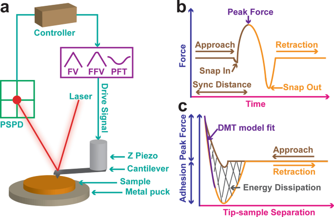
AFM 力斜坡机制、实验设计、数据采集和解释。 LDPE 样品安装在金属圆盘上。锋利的悬臂尖端压入 LDPE 样品中，并在达到预设的施加力时缩回 (a ）。一束激光从顶部射出，击中并从悬臂的背面偏转。偏转信号由位置敏感光电二极管 (PSPD) 接收。悬臂运动由连接的 Z 压电驱动。根据技术的选择，驱动信号可以是三角波 (FV)、圆角三角波 (FFV) 或正弦波 (PFQNM)。 b 中示意性地描述了 PFQNM 力测量 ，力与时间图清楚地说明了尖端在靠近样品表面时经历了咬合接触，而在远离样品表面时会发生接触。同步距离是高度传感器到达最低位置的时间常数。力与 Z 位移曲线 (F-Z) 由 AFM 记录并进一步转换为力与尖端-样品分离 (F-D) 曲线 (c ）。通过用DMT模型拟合回缩曲线的接触部分来提取DMT模量。磁滞回线上的积分称为能量耗散

数据分析

使用 AFM 工厂提供的 NanoScope 分析软件 (Bruker Co., Santa Barbara, CA) 进行离线数据分析。所有地形图像都经过一阶平坦化处理，以消除 Z 压电漂移、背景噪声以及校正样本倾斜。表面粗糙度通过NanoScope Analysis软件提供的表面粗糙度特征评价。

其中 \(N\) 是图像区域内的点总数，\(Z_{{\text{i}}}\) 是 i 的 \(Z\) 高度 第一个数据点，\(Z_{{\text{m}}}\) 是整个区域的平均 \(Z\) 高度。所有机械数据图像均保持原样，未整平。

力斜坡、快速力体积和 PFQNM 均产生力与 Z 压电位移 (F-Z) 曲线。力与尖端样品分离 (F-D) 曲线在物理上更有意义，并且需要模型拟合。 Z 位移由三个分量组成，即尖端-样品分离 (D ), 悬臂挠度 (d ) 和压痕深度 (\(\delta\))。 F-Z 到 F-D 的转换需要减去悬臂挠度 (d )，以及来自 Z 位移的压痕深度 (\(\delta\))。它可以在实时控制软件或离线数据分析软件中完成，前提是悬臂挠度灵敏度和弹簧常数已经校准。此外，执行基线校正功能将力曲线基线偏移为零。最后，获得 F-D 曲线并进行 DMT 模型拟合。根据赫兹接触理论，

其中 \(F_{{{\text{appl}}}}\) 是尖端施加在样品上的力。粘附力 (\(F_{{{\text{adh}}}}\)) 被考虑在内。 \(R\) 是假定球体尖端的尖端半径。 \(\delta\) 是压痕深度。 \(E_{{\text{r}}}\) 是减少的杨氏模量。它与tip和sample的模量有关，

其中 \(v_{{\text{s}}}\) 和 \(v_{{\text{t}}}\) 分别是样本和 AFM 尖端的泊松比。 \(E_{{\text{s}}}\) 和 \(E_{{\text{t}}}\) 分别是样本和 AFM 尖端的杨氏模量。尖端的杨氏模量比 LDPE 样品的杨氏模量大几个数量级，因此尖端项可以忽略。一旦\(E_{{\text{r}}}\) 和\(v_{{\text{s}}}\) 已知，\(E_{{\text{s}}}\) 可以很容易地计算。

通过采取等式的两边。 (3) 将 \(F_{{{\text{appl}}\) 减去 \(F_{{{\text{adh}}}}\) 后的 \(\frac{2}{3}\) 幂}}\)，一个线性模型被用来拟合所有的力数据[30]。该模型不需要识别接触点。

然后 \(E_{{\text{r}}}\) 和 \(E_{{\text{s}}}\) 被提取出来。

由于悬臂的作用类似于弹簧，因此施加的力由胡克定律计算。

其中\(k\)为悬臂弹簧常数，\(d\)为悬臂挠度，由悬臂挠度灵敏度乘以垂直挠度信号计算得出。

对于蠕变柔量分析，采用了 Voigt 版本的 SLS 模型[19]。在这个三元素模型中，弹簧 (E 1) 与弹簧 (E 2)-并联缓冲器Voigt元件。压缩距离 (d ) 作为时间的函数可以描述为：

其中 F 是总加载力，k 1 和 k 2 是 E 的弹性 1 和 E 2、分别。 η 代表缓冲器的粘度。由于尖端-样品相互作用区域是一个有限区域，而不是单个点。可以通过在应力、应变和模量方面重写方程来改进模型。本研究采用了 Lam 及其同事开发的方法。它们的类似等式是：

其中 ε (t ) 表示作为函数时间的应变，σ 是压力。 E 1 和 E 2 分别是瞬时弹性模量和延迟弹性模量。 η 代表缓冲器的粘度。此外，应力σ 和应变 ε 与模数 E 相关 或合规性D 由以下关系。

因此等式 (9) 可以改写为：

其中 D 和 E 分别表示系统的蠕变柔量和组合弹性模量。重写方程。 (5) 如

代入方程。 (11) 进入方程。 (12) 引起

蠕变数据可以拟合方程。 (13) 和延迟时间τ 可以使用

延迟时间是指发生 ~ 63%蠕变的时间。

所有力测量均重复 3 次。结果以平均值 ± SD（标准偏差）的形式报告，而独立实验的数量表示为n =3.

结果

为了评估 PFQNM 的有效性和准确性，进行了 5 µm × 5 µm 的大型调查扫描。图 2 中组装了 2 kHz 下 PS/LDPE 混合样品的代表性 PFQNM 图像。图 2a-d 是高度传感器图像、DMT 模量通道、压痕通道和能量耗散通道。平坦区域是 PS 组件，而凸出区域是 LDPE（图 2a）。完成勘测扫描后，AFM 被指示物理放大 LDPE 区域并进行高分辨率小尺寸 (1.3 µm × 1.3 µm) 扫描。相应的图像通道显示在图 2e-h 中。

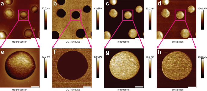
PS/LDPE 混合样品在 2 kHz 时的代表性 PFQNM 纳米力学映射（5 µm × 5 µm）。面板a –d 是高度传感器图像、DMT 模量通道、压痕通道和能量耗散通道。对于图像a –d ，比例尺代表 1 µm。完成勘测扫描后，AFM 被引导物理放大 LDPE 区域并进行高分辨率小尺寸 (1.3 µm × 1.3 µm) 扫描。相应的图像通道显示在面板 e–h 中 .比例尺代表面板 e 的 260 纳米 –h

接下来，PFQNM、FV 和 FFV 在 0.5 µm × 0.5 µm 的纯 LDPE 区域上进行。在图 3a-d 中收集了一组 2 kHz 的代表性 PFQNM。它们包括高度传感器、模量映射、能量耗散和压痕。高度传感器图像的表面粗糙度以 \(R_{{\text{q}}}\) 的形式报告为 2.58 ± 0.35 nm。图 3e、f 中显示了 122 Hz 下的另一组代表性 FFV。请注意，FV 和 FFV 没有能量耗散和压痕通道。不同频率的弹性模量汇集在一起​​（图 3g）。杨氏模量数据在表 1 中报告。杨氏模量在 0.1 Hz、1 Hz、10 Hz、20 Hz、61 Hz、122 Hz、125 Hz、250 Hz、500 Hz、1 k Hz 和 2 k 7 Hz 时为 ≡ 11 ± 11 ±。 5.2 兆帕 (n =3), 18.2 ± 5.6 MPa (n =3), 25.4 ± 6.8 MPa (n =3), 29.6 ± 8.4 MPa (n =3), 33.8 ± 9.7 MPa (n =3), 35.7 ± 10.5 MPa (n =3), 43.8 ± 10.7 MPa (n =3), 54.8 ± 11.9 MPa (n =3), 66.7 ± 13.6 MPa (n =3), 80.9 ± 14.2 MPa (n =3), 89.6 ± 17.3 MPa (n =3)，分别。散点图由Origin 8.5软件生成。用幂函数拟合数据，得到\(E =15.31 \times f^{{0.23}}\) (\(R^{2}\) =0.96)。能量耗散与不同映射频率之间的关系绘制在图 3h 中。在 2 kHz、1 kHz、0.5 kHz、0.25 kHz 和 0.125 kHz 下获得的能量耗散值为 173.2 ± 21.9 eV (n =3), 213.8 ± 32.7 eV (n =3), 233.9 ± 29.3 eV (n =3), 261.1 ± 33.5 eV (n =3), 293.2 ± 35.6 eV (n =3)，分别。数据用幂函数拟合得到 \(E_{{{\text{diss}}}} =202.83 \times f^{{ - 0.18}} ~\) (\(R^{2}\) =0.97 ）。代表性 F-D 曲线显示 AFM 尖端与 LDPE 样品表面有两个明显的破裂（图 3i）。多次破裂的发生频率较低，即 0.1–1 Hz。

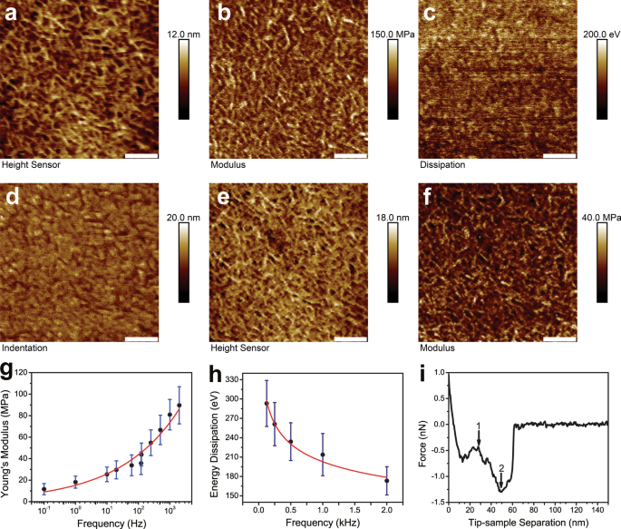
LDPE 样品在不同频率下的力学性能映射。面板a –d 是高度传感器图像、DMT 模量通道、能量耗散和用 PFQNM 在 2 kHz 下在纯 LDPE 区域捕获的压痕通道。高度传感器图像的表面粗糙度以 \(R_{{\text{q}}}\) 的形式报告为 2.58 ± 0.35 nm。面板 e 和 f 是高度传感器图像和 DMT 模量通道，在 122 Hz 的 FFV 下在纯 LDPE 区域捕获。对于图像a –f ，比例尺代表 100 nm。测得的杨氏模量 (E ) 和力映射频率 (f ) 在 g 中绘制 .不同频率下测得的杨氏模量如表 1 所示。数据拟合幂函数得到 \(E =15.31 \times f^{{{0.23}}\) (\(R^{2}\) =0.96 ）。能量耗散 (E diss) 和不同的映射频率 (f ) 显示在面板 h 中 .在 2 kHz、1 kHz、0.5 kHz、0.25 kHz 和 0.125 kHz 下获得的能量耗散值分别为 173.2 ± 21.9 eV、213.8 ± 32.7 eV、233.9 ±3 3.7eV、233.9 ±3 3.5.3 3.5.3≉±3.5.3≉±3.5.3≉3.5 The data were fitted with a power function yielded \(E_{{{\text{diss}}}} =202.83 \times f^{{ - 0.18}} ~\) (\(R^{2}\) = 0.97). A representative F-D curve showed two distinct ruptures of AFM tip from LDPE sample surface (panel i ）。 The occurrence of multiple ruptures took place more frequently at lower frequencies, i.e. 0.1–1 Hz

Lastly, creep compliance measurement was carried on a neat LDPE region of the PS/LDPE sample. The working principle of AFM creep experiment was illustrated in Fig. 4a. Initially, the AFM tip was brought into contact with sample surface until the predefined force setpoint was reached. The tip was sthen held onto the sample for a certain time period, during which the force was kept constant. Following that, the tip was retracted. In the hold segment, the AFM recorded the change in Z motion. The change in indentation depth as a function of time (Fig. 4b) could be fitted with Voigt version of SLS model using Eq. (13). A representative creep curve was shown in Fig. 4c. The black curve was the data while the red solid line was the fitting curve. The inset indicated the Voigt version of SLS model, featuring a spring (E 1) in series with a spring (E 2 )-dashpot (η ) Voigt element in parallel. The experiment showed that instantaneous elastic modulus E 1, delayed elastic modulus E 2, viscosity η , retardation time τ were 22.3 ± 3.5 MPa, 43.3 ± 4.8 MPa, 38.7 ± 5.6 MPa‧s and 0.89 ± 0.22 s, respectively. The data were tabulated in Table 2.

Creep compliance measurement on a neat LDPE region of the PS/LDPE sample. The working principle of AFM creep experiment was illustrated in panel a . Initially, the AFM tip was brought into contact with sample surface till it reached the predefined force setpoint. The tip was then held onto the sample for a certain time period, during which the force was kept constant. Following that, the tip was retracted. In the hold segment, the AFM recorded the change in Z motion (panel b ）。 The change in indentation depth as a function of time could be fitted with Voigt version of SLS model using Eq. (13). A representative creep curve was shown in panel c . The black curve was the data, while the red solid line was the fitting curve. The inset indicated the Voigt version of SLS model, featuring a spring (E 1) in series with a spring (E 2)-dashpot (η ) Voigt element in parallel

Discussion

In the present study, a comprehensive powerful nanomechanical mapping approach for polymer samples has been developed by incorporating a number of nanoscale AFM based force measurements. The approach allows simultaneous high-resolution topography imaging and quantitative nanomechanical mapping. Local mechanical behavior can be correlated with sample topography. More importantly, the time dependent mechanical response of soft viscoelastic materials has been successfully mapped out. The Hertz model is a widely received contact mechanics model [31], in which the scenario when a rigid probe indents a semi-infinite, isotropic, homogeneous elastic surface is described. However, the Hertz model assumes no surface forces, which is not true for soft materials. To overcome this shortcoming, the Johnson–Kendall–Roberts (JKR) model and the DMT model have been developed. Given the setup in this study, the DMT model can be implemented as there are high elastic modulus, low adhesion, and small tip radius involved where long rang surface forces exist. The force setpoint at 5 nN has been empirically obtained, and justified to be the optimum value in terms of getting meaningful indentation depth while the DMT model still holds. Low force load also gives rise to sample deformation in elastic regime not plastic regime. In addition, sharp tip enables high resolution sample topography imaging in PFQNM measurements, which is an attractive advantage when correlates sample topography with mechanical properties.

Tip radius estimation is not trivial in quantitative mechanical measurements. Many researches estimate the tip radius by backward calculation using a sample with known modulus [29, 32]. This work adopts a different reconstruction strategy that does not require such a sample. It has been documented that using blunt tips tend to yield tighter modulus numbers and that sharp tips may overestimate the modulus. However, sharp tips preserve high spatial resolution, an advantage not possessed by other techniques. Polymer fibrils are clearly seen (see a 0.5 µm × 0.5 µm scan in Fig. 3). Sharp tips, even under small load, can penetrate into compliant samples due to large stress, resulting in large indentation. Therefore, it could compromise the validity of the DMT model. That is not the case in this study as the applied force is controlled in a precise and sensitive manner, evidenced by the resulted indentation depth and the effective tip radius in the same order of magnitude (22.5 ± 3.2 nm, n =3)。 Surface roughness (\(R_{{\text{q}}}\)) of the LDPE height image is 2.58 ± 0.35 nm, indicating the surface is flat and surface roughness should not be treated as a confounding factor to quantitative measurements [33]. In addition, the linearized DMT model fit does not require determination of the contact point that could otherwise lead to major errors in the final calculated modulus [34]. Taken together, the current experiment setup fulfills the DMT model.

To evaluate the effectiveness of PFQNM, the PS/LDPE sample has been scanned at large size. The survey scan shows LDPE has higher adhesion than PS (Fig. 2b), suggesting LDPE is stickier. AFM tip indents deeper in LDPE than in PS (Fig. 2c), indicating LDPE is softer than PE. The determined Young’s moduli for LDPE and PS are about 90 MPa and 2.5 GPa, respectively. The PS region is a little stiff for RTESPA-150 probe to indent, thus the measured modulus tends to be higher than the nominal value. Both PFQNM and FFV generate high resolution topography and modulus images (c.f. Fig. 3a, b, e, f). It is noteworthy that FFV requires reasonable data acquisition time, although it is not as impressive as PFQNM but much faster than traditional force ramp. Energy dissipation is an observable that explicitly demonstrates how much energy loss per tapping cycle (Fig. 3h). The more viscoelastic of the material, the more energy loss it incurs. The energy dissipation map demonstrates that AFM probe loses more energy on LDPE than on PS, implying LDPE is viscoelastic and response time plays an important role. The relaxation function for the power-law rheology model is described as \(\varphi =E_{{\text{a}}} \left( {\frac{t}{{t_{0} }}} \right)^{{ - \gamma }}\) [35], where E a is the apparent Young’s modulus at time t 0, is the power-law exponent γ 和 t 0 is a timescale factor which is set to 1 s. The dimensionless number γ characterizes the viscoelastic behavior of the material, with γ  = 0 for purely elastic solid and γ  = 1 for purely Newtonian fluid [36]. Current study indicates LDPE has more elastic behavior than viscous counterpart. Figure 3i exhibits an interesting finding in FV experiments that a force curve harboring two rupture events. The multiple rupture events occur more frequently in lower frequencies, i.e. 0.1–1 Hz. It is conceivable that with lower frequency, the tip dwells longer on sample surface that results in forming stronger bonds. When tip is retracted, the slower motion of tip would break the bonds at lower speed, providing the chance of being captured by AFM [37]. On the contrary, when performed at higher frequencies, weaker bonds are formed due to short dwell period and AFM is not capable of capturing transition rupture events due to poor temporal resolution. Another plausible explanation is that the combination of force exerted and longer interaction time on sample induces polymer chain conformation change, as reported previously that force induces rotation of carbon–carbon double bonds [38]. With piconewton force sensitivity and sub-nanometer distance accuracy, F-D curves not only reveal the strength of the formed bonds but also shed insights into the elastic properties and conformational changes. It was documented that at low forces (< 100 pN) and large forces (> 300 pN) the mechanical behavior of polymer chains is majorly affected by its entropic elasticity and enthalpic elasticity, respectively [39].

To further investigate the time dependent mechanical response of LDPE, creep compliance experiment has been carried out on the premise that the closed-loop scanner has been drift calibrated. Experimental data show that instantaneous elastic modulus E 1, delayed elastic modulus E 2, viscosity η , retardation time τ are 22.3 ± 3.5 MPa, 43.3 ± 4.8 MPa, 38.7 ± 5.6 MPa s and 0.89 ± 0.22 s, respectively (Table 2). This set of values for creep behavior is close to those reported for polyurethane nanocomposites [40] and syndiotactic polypropylene [41] and higher than those for bacterial biofilm [19] and live cells [36, 42]. While large AFM indenter platform measures elastic modulus of soft samples in an ensemble way, it does not enjoy high spatial resolution of elasticity. Such local mechanical properties are critical for some specimen. For instance, cell membranes are composed of various substructures like cytoskeleton, filament network and microvilli, each has varying elasticities [30]. A recent paper has studied the elastic modulus of fibroblast cells in the frequency range of 0.3–250 Hz [43]. The authors have discovered raised apparent Young’s modulus when ramp frequency increased, consistent with the observations of current study. The approaches reported here are as reliable as any other nanomechanical techniques provided the force-indentation has been prudently designed and the data analysis has been carefully executed. The PFQNM measurement is particularly helpful due to its localized correlation of sample topography with mechanical behavior. It is advantageous in terms of local non-destructive probing of mechanical properties over traditional instrumented indentation, where large probe tip is used and large destructive force is applied. Furthermore, the AFM creep experiment provides dynamic mechanical behavior at nanoscale. The methodology presented here offers multiparametric, multifunctional probing of mechanical measurement along with exceptional high spatial resolution. It has been successfully exploited for quantitative nanomechanical mapping of soft polymers such as LDPE, and can potentially be extended to complex biological systems [43,44,45].

结论

Utilizing state-of-the-art PFQNM as well as with FV and FFV, the power-low rheology of a LDPE sample has been evaluated in a time-dependent fashion. Specifically, rigorous calibrations are done. Force data are fitted with a linearized DMT contact mechanics model considering surface adhesion force. Elastic Young’s modulus was measured at frequencies spanned four orders of magnitude. Increased Young’s modulus was discovered with increasing acquisition frequency. The Young’s modulus is 11.7 ± 5.2 MPa at 0.1 Hz but increases to 89.6 ± 17.3 MPa at 2 kHz. The acquisition frequency dependent modulus change could be described by a power function \(E =15.31 \times f^{{0.23}}\) (\(R^{2}\) = 0.96). Energy dissipation in the range of 0.125–2 kHz further supports this observation. Furthermore, creep compliance experiment shows that instantaneous elastic modulus E 1, delayed elastic modulus E 2, viscosity η , retardation time τ are 22.3 ± 3.5 MPa, 43.3 ± 4.8 MPa, 38.7 ± 5.6 MPa‧s and 0.89 ± 0.22 s, respectively. The multiparametric, multifunctional local probing of mechanical measurement along with exceptional high spatial resolution imaging open new opportunities for quantitative nanomechanical mapping of soft polymers, and can potentially be extended to biological systems.

数据和材料的可用性

本研究中使用或分析的数据集可向相应作者索取。

缩写

原子力显微镜：

原子力显微镜

DMT:

Derjaguin–Muller–Toporov

FFV:

Fast force volume

FV:

Force volume

JKR:

Johnson–Kendall–Roberts

LDPE:

Low density polyolefin

PFQNM:

PeakForce quantitative nanomechanical mapping

PFT:

PeakForce tapping

附注：

聚苯乙烯