工艺过程的过程控制

工艺流程控制

技术过程包括处理、加工、精炼、组合和操纵材料和流体，以有利地生产最终产品。这些过程可能是精确的、苛刻的和潜在危险的过程。过程中的微小变化会对最终结果产生很大影响。对比例、温度、流量、湍流和许多其他参数的变化进行仔细和一致的控制，以始终如一地以最少的原材料和能源生产出所需质量的最终产品。

通常，任何需要对操作进行持续监控的事情都涉及过程控制的作用。过程控制是指用于控制工艺过程的过程变量的方法。它是一种工具，使流程能够使流程操作在指定的范围内运行，并设置更精确的限制，以最大限度地提高流程效率，确保质量和安全。

每个工艺流程都需要大量的计划才能成功完成其既定任务。然而，为了完成这些任务，过程操作员必须充分了解过程和控制系统的功能。控制系统由设备（测量装置和控制装置等）以及操作员的干预组成。控制系统用于满足过程的三个基本需求，即（i）减少外部干扰的影响，（ii）促进过程的稳定性，以及（ii）提高过程的性能。

仪表提供用于操作技术过程的各种指示。在某些情况下，操作员会记录这些指示以用于过程操作。记录的信息有助于操作员评估过程的当前状况，并在状况不符合预期时采取措施。要求操作员采取所有必要的纠正措施是不切实际的，有时甚至是不可能的，尤其是在要监测大量迹象的情况下。因此，大多数工艺流程一旦在正常条件下运行，就会自动控制。自动控制大大减轻了操作员的负担，使工作易于管理。技术过程受到控制的三个原因是：(i) 减少可变性，(ii) 提高效率，以及 (iii) 确保安全。

过程控制可以减少最终产品的可变性，从而确保始终如一的高质量产品。随着工艺可变性的减少，工艺变得更加稳定、可靠、高效和经济。一些工艺参数将保持在特定水平，以最大限度地提高工艺效率。对这些参数的准确控制可确保过程效率。此外，如果在过程操作过程中没有保持对所有过程变量的精确控制，则可能导致失控过程，例如失控的化学反应。失控过程的后果可能是灾难性的。因此，还需要对过程进行精确控制，以确保设备和工人的安全。

多年来，过程控制的作用发生了变化，并且不断受到技术的影响。过程控制的传统作用是通过将过程变量保持在所需值附近来促进安全、最大限度地减少对环境的影响并优化过程。过去，工艺参数的监控是在工艺现场进行的，并且这些参数由操作员在本地进行维护。随着流程规模变得更大和/或更复杂，流程自动化的作用变得越来越重要。今天自动化已经接管了过程控制功能，这意味着操作员可以通过计算机分布式控制系统（DCS）与现场的仪器进行通信。

过程控制是统计学和工程学科的混合体，它处理控制过程的机制、架构和算法。要进行有效的过程控制，除了了解过程技术外，还需要了解过程控制的关键概念和通用术语。

控制过程的原因是让它以所需的方式运行。这可能涉及过程变得更准确、更可靠或更经济。在某些情况下，不受控制的过程是不稳定的，为了不损坏它，必须进行良好的控制。因此，良好的控制在不同的应用中可能意味着不同的东西。

在过程控制中，基本目标是调节某个参数的值。调节意味着无论外部影响如何，都将参数的数量保持在某个期望值。所需的值称为参考值或设定点。 操作员可以改变设定点。如果通过改变输入设定点，输出改变以匹配输入设定点，则该过程是自我调节的。 . 自调节系统不提供对任何特定参考值的变量调节。该参数采用输入和输出值相同的某个值，并保留在那里。但是如果输入流量发生变化，那么输出也会发生变化，所以没有调节到一个参考值。

操作员辅助控制允许操作员进行人工调节。为了调节参数，使其保持所需的值，需要一个传感器来测量参数。该参数称为控制变量。 通过操作合适的控制设备，操作员可以将输出参数更改为设定值。输出参数称为操作变量或控制变量。

自动控制系统取代了控制系统，并使用机器、电子设备或计算机来取代操作员的操作。添加了一种称为传感器的仪器，该仪器能够测量参数的值并将其转换为比例信号。该信号作为输入提供给称为控制器的机器、电子电路或计算机。 控制器在评估测量和提供输出信号时执行操作员的功能, 通过机械联动装置连接到设备的执行器更改控制设备设置。当自动控制应用于旨在将某些变量的值调节到设定点的系统时，称为自动过程控制。 Fig1 以框图形式展示了输入输出变量的概念控制过程。

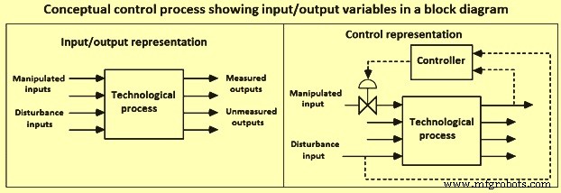
图 1 在框图中显示输入输出变量的概念控制过程

技术过程本质上是动态的，因为它们很少在稳定状态下运行。工艺流程的操作包括确保对不断发生的干扰做出适当的响应，以确保操作安全、高效，并以所需的速率生产具有指定质量的所需产品。由于生产方法因过程而异，因此自动控制的原理本质上是通用的，可以普遍应用，无论过程的大小和类型如何。过程控制系统的目标是执行以下一项或两项任务。

将过程保持在操作条件和设定点 – 许多过程需要在稳定状态条件下或在满足成本、产量、安全和其他质量目标等所有要求的状态下工作。在许多现实生活中，一个过程不可能总是保持静止，并且过程中会发生一些干扰，从而使过程不稳定。在不稳定的过程中，过程变量会在有限的时间跨度内从其物理边界振荡。不受控制的过程变量可以通过添加控制仪器和设备来控制，这些控制仪器和设备可以自动或通过操作员的干预将过程变量控制在其控制范围内。

将流程从一种操作条件转换到另一种操作条件 – 在现实生活中，由于各种不同的原因，有时需要改变工艺操作条件。将工艺从一组操作条件转换到另一组操作条件的原因可能是由于经济性、产品规格、操作限制、环境法规和产品规格变化等。

技术过程控制策略的开发包括制定或识别 (i) 控制目标，(ii) 输入变量，这些输入变量可以是操纵变量或干扰变量，并且可以连续或以离散的时间间隔变化， (iii) 可以是测量变量或未测量变量的输出变量，可以连续或以离散的时间间隔测量，(iv) 可以是硬的或软的约束，(v) 可以是批量的操作特性，连续或半连续，(vi) 安全、环境和经济考虑，以及 (vii) 控制器可以在本质上反馈或前馈的控制结构。一个工艺过程的过程控制系统的制定包括七个阶段。

开发控制系统的第一阶段是制定控制目标。工艺流程通常由几个子流程组成。单独考虑各个子过程的控制时，工艺过程的控制就减少了。即使这样，每个子过程也可能有多个，有时是相互冲突的目标，因此控制目标的制定通常是一个困难的问题。

第二阶段构成输入变量的确定。输入变量显示环境对过程的影响。它通常是指影响过程的那些因素。输入变量可分为操纵变量或干扰变量。受控输入是可以由控制系统（或过程操作员）调整的输入。干扰输入是影响过程输出但不能由控制系统调整的变量。存在可测量和不可测量的干扰输入。输入可以连续变化，也可以不连续的时间间隔变化。

第三阶段构成输出变量的确定。输出变量也称为控制变量。这些是影响周围环境的过程输出变量。输出变量可以分为测量变量或未测量变量。测量可以连续进行，也可以不连续的时间间隔进行。

第四阶段构成操作约束的确定。每个流程都有一定的操作约束, 分为硬的或软的。硬约束的示例是阀门在完全关闭或完全打开的极端条件之间运行的最小或最大流速。软约束的示例是产品成分，希望在一定范围内指定成分，但在不构成安全或环境危害的情况下违反此规范是可能的。

第五阶段构成操作特性的确定。操作特性通常分为间歇式、连续式或半连续式。连续过程在相对恒定的操作条件下长时间运行，然后“关闭”以执行某些工作，例如清洁和定期预防性维护等。批处理过程本质上是动态的，也就是说，它们通常运行很短的时间在这段时间内，运行条件​​可能会发生很大变化。批处理示例是在炼钢炉中加热。对于间歇式反应器，对反应器进行初始装料，并改变工艺条件以在间歇式工艺结束时生产所需的产品。典型的半连续过程可以对反应器进行初始进料，但进料组分可以在分批运行过程中添加到反应器中。连续铸造工艺是半连续工艺的例子。一个重要的考虑因素是该过程的主要时间尺度。对于连续过程，这通常与材料在反应器中的停留时间有关。

第六阶段是关于安全、环境和经济问题的重要考虑。从某种意义上说，经济是最终的驱动力，因为不安全或对环境有害的过程最终会因为监管处罚和效率低下而增加运营成本。此外，重要的是在生产符合规格的产品时尽量减少能源成本。更好的流程自动化和控制允许流程更接近“最佳”条件运行，并生产出满足可变性规范的产品。

“故障安全”的概念在选择仪器时始终很重要。例如，控制阀需要一个能源来移动阀杆并改变流量。最常见的是气动信号（通常为 3 -15 PSI）。如果信号丢失，则阀杆达到 3 PSI 限制。如果阀门是“气开”，那么仪表空气的损失会导致阀门关闭，这被称为“故障关闭”阀门。另一方面，如果阀门是空气关闭，当仪表空气丢失时，阀门会进入完全打开状态，这被称为“故障打开”阀门。

有两种标准控制类型，即（i）前馈控制和（ii）反馈控制。前馈控制器测量扰动变量并将该值发送到控制器，控制器调整受控变量。反馈控制的目的是使受控变量接近其设定点。反馈控制系统测量输出变量，将该值与所需的输出值进行比较，并使用此信息来调整操作变量。通过其设计，反馈控制器采取纠正措施来减少偏差。反馈控制器只能在受控变量偏离其所需设定点并产生非零误差后才能采取行动。但是，如果过程或测量变化非常缓慢，则对干扰的响应可能非常缓慢。在这种情况下，前馈控制器可以提高性能。前馈控制器预测扰动对被控变量的影响，并采取控制措施抵消扰动的影响。

确定过程的反馈控制结构包括决定调整哪个操作变量以控制哪个测量变量。测量过程输出的期望值称为设定点。受控变量偏离其设定点有两个原因。为了获得更好的性能或干扰驱使操作远离其所需的设定点，故意更改设定点。设计用于抑制干扰的控制器称为调节器，而设计用于跟踪设定点变化的控制器称为伺服机构。通常对于连续过程，设定点变化很少发生，通常只有在监督控制器计算出更有利的操作点时，因此，调节器是最常用的反馈控制器形式。相比之下，伺服问题控制器在批处理过程中很常见，其中设定点经常发生变化。

控制系统设计中使用的一个特别重要的概念是“过程增益”。 “过程增益”是过程输出对过程输入变化的敏感度。如果过程输入的增加导致过程输出的增加，这称为正增益。另一方面，如果过程输入的增加导致过程输出的减少，这称为负增益。 “过程增益”的大小也很重要。

一旦确定了控制结构，就必须决定控制算法。控制算法使用测量的输出变量值（连同所需的输出值）来改变受控输入变量。控制算法具有许多控制参数，这些参数要被调整以具有可接受的性能。在对实际过程实施控制策略之前，通常会在模拟模型上进行调整。在基于模型的控制的情况下，控制器具有“内置”过程模型。

具有单个操纵变量和单个受控变量的工艺过程框图（图 2）包括前馈、反馈和监督控制。反馈控制器的主要目的是使由某些仪器测量的受控变量 X 尽可能接近所需的设定点 Xsp。控制变量可以是工艺过程的任何参数。设定点通常由监控系统使用实时数值优化技术确定。有几种不同类型的最终控制元素。扰动变量 D，也称为负载变量，可导致受控变量偏离其设定点，需要采取控制措施以使其回到所需的工作点。反馈和前馈控制都可以减少干扰的影响，每种方法都有其优点和缺点。干扰可能来自多种来源，包括外部环境变量。在任何情况下，干扰变量都不会受到过程控制器的影响。受控变量 X 与其设定点 Xsp 之间的误差或偏差 E 是反馈控制器的输入，它改变操纵变量 M 以减小误差。在一个典型的工艺流程中，可以有大量这样的控制回路。

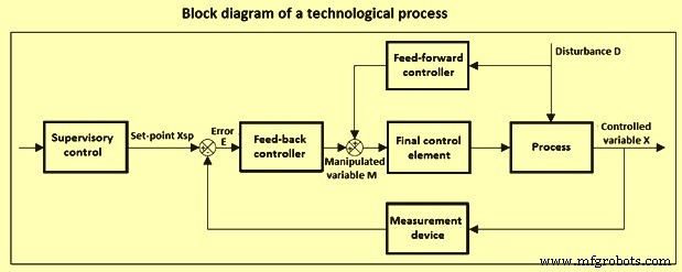
图2工艺流程控制框图

控制硬件和软件

自 1940 年代首次引入以来，过程工业中实施的过程控制已经发生了重大变化。在 1960 年代初期，电气模拟控制硬件取代了大部分气动模拟控制硬件。然而，在许多过程中，某些控制元件，即控制阀执行器，即使在今天仍然保持气动。 1960 年代的电气模拟控制器是单回路控制器，其中每个输入首先从过程中的测量点带到大多数控制器所在的控制室。然后控制器的输出从控制室发送到最终控制元件。操作员界面由一个控制面板组成，该控制面板结合了显示面板和用于单回路控制器和指示器的图表记录器。控制策略主要涉及反馈控制，通常使用比例积分 (PI) 控制器。在 1950 年代末和 1960 年代初，引入了用于执行直接数字控制 (DDC) 和监督过程控制的过程控制计算机。在使用 DDC 的情况下，DDC 回路通常具有接近 100 % 的模拟控制备份，这使得系统成本很高。

其他早期系统主要使用过程控制计算机进行监督过程控制。监管控制由模拟控制器提供，不需要备份，但操作员的注意力分散在控制面板和计算机屏幕之间。使用监控时，终端显示器提供操作员界面，但在需要模拟备份时，控制面板仍位于控制室中。在这种环境下，前馈控制、多变量解耦控制和串级控制等先进控制技术得到了广泛应用。这些早期控制系统的功能是围绕计算机的功能而不是过程特性设计的。这些限制，加上操作员培训不足和用户界面不友好，导致设计难以操作、维护和扩展。此外，许多不同的系统都有定制的规格，因此非常昂贵。 1970 年左右，当廉价的微处理器开始商业化时，数字系统应用程序被注入到过程工业中。

分布式控制系统 (DCS) – DCS 由许多元素组成，如图 3 所示。主机执行计算密集型任务，如优化和高级控制策略。由数字传输链路组成的数据高速公路连接系统中的所有组件。冗余数据高速公路减少了可能的数据丢失。操作员控制站为操作员与系统通信提供视频控制台，以监督和控制过程。许多控制站包含用于报警记录、报告打印或过程图形硬拷贝的打印机。远程控制单元实现 PID 算法等基本控制功能，有时还提供数据采集功能。程序员控制台为分布式控制系统开发应用程序。大容量存储设备存储用于控制目的以及公司决策的过程数据。存储设备可以是硬盘或数据库的形式。控制器、输入和输出之间的通信和交互是通过软件实现的，而不是通过硬件实现的。因此，DCS 彻底改变了过程控制的许多方面，从控制室的出现到先进控制策略的广泛使用。

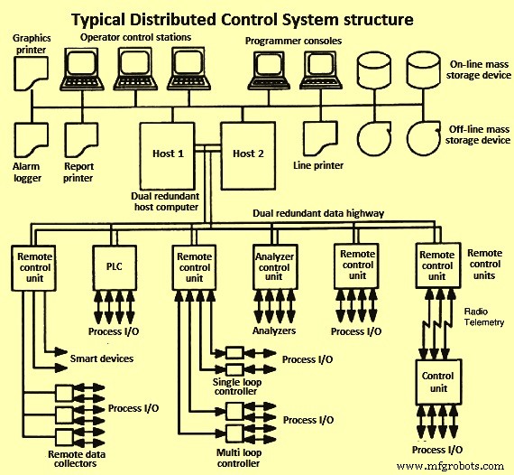
图3 DCS系统典型结构

可编程逻辑控制器 (PLC) – 最初，PLC 控制器是专用的、独立的、基于微处理器的设备，执行简单的二进制逻辑以进行排序和联锁。 PLC 显着提高了对此类逻辑进行修改和更改的便利性。 PLC 在计算能力方面变得越来越强大。批处理控制以逻辑类型控制为主，PLC 是 DCS 的首选替代方案。由于 DCS 和 PLC 之间具有相对平滑的集成接口，目前的做法通常是使用 DCS 和 PLC 的集成组合。大多数 PLC 还处理时序逻辑，并配备了内部定时功能，可以将动作延迟规定的时间，在规定的时间内执行动作，等等。

安全和关闭系统 – 过程控制在过程的安全考虑中起着重要作用。当自动化程序取代日常操作的手动程序时，导致危险情况的人为错误的可能性变得更小。此外，操作员对当前工厂状况的认识也得到了提高。应为危险的 e 过程提供保护系统。一种方法是为特定目的提供逻辑，以将过程带到不存在这种情况的状态，称为安全联锁系统。由于过程控制系统和安全联锁系统的用途不同，因此它们在物理上是分开的。它降低了无意更改安全系统的风险。已经为安全停机开发了特殊的高可靠性系统，例如三重模块化冗余系统。这允许系统发生内部故障并仍然执行其基本功能。基本上，三重模块化冗余系统由三个相同的子系统组成，同时主动执行相同的功能。

警报 – 警报的目的是提醒过程操作员注意需要立即注意的过程条件。只要检测到异常情况并发出警报，就会激活警报。当异常情况不再存在时，报警恢复正常。可以在测量变量、计算变量和控制器输出上定义警报。存在多种不同类别的警报。

智能变送器、阀门和现场总线 – 过程控制技术有一个明确的趋势，即越来越多地使用数字技术。数字通信发生在现场总线上，即同轴或光纤电缆，智能设备直接连接到现场总线，并作为数字信号与控制室或远程设备室进行传输。现场总线方法减少了对双绞线和相关布线的需求（图 4）。

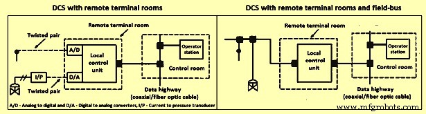
图 4 带有远程房间终端和现场总线的 DCS

各种现场网络协议提供了在现场设备、仪器和控制系统之间传输数字信息和指令的能力。现场总线软件调解组件之间的信息流。多个数字设备可以通过数字通信线相互连接和通信，大大减少了布线。

过程控制软件 – 最广泛采用的用户友好方法是填写表格或表格驱动的过程控制语言 (PCL)。流行的 PCL 包括功能块图、梯形逻辑和可编程逻辑。这些语言的核心是一些基本的功能块或软件模块，如模拟输入、数字输入、模拟输出、数字输出、PID等。一般来说，每个模块包含一个或多个输入和一个输出。编程涉及通过图形用户界面将块的输出转换为其他块的输入。用户需要填写模板来指明输入值的来源、输出值的目的地以及为模块准备的表格/表格的参数。源和目标空白可以在适当的时候指定进程 I/O（输入/输出）通道和标签名称。为了连接模块，某些系统需要填写发起或接收数据的模块的标签名称。用户指定的字段包括特殊功能、选择器（最小值或最大值）、比较器（小于或等于）和计时器（激活延迟）。大多数 DCS 允许创建功能块。

设施控制层级 – 采用各种优化、控制、监控和数据采集活动的工艺过程中的五个层次如图 5 所示。图中每个块的相对位置是概念性的，因为在图 5 中可能存在重叠执行的功能。还显示了每个级别处于活动状态的相对时间尺度。五个概念控制级别中的每一个在硬件、软件、技术和定制方面都有自己的要求和需求。因为信息在层次结构中向上流动而控制决策向下流动，所以只有当关注级别之下的所有级别都运行良好时，特定级别的有效控制才会发生。最高级别（计划和调度）设定生产目标以满足供应和物流限制，并解决随时间变化的产能和人力利用决策。这称为企业资源计划 (ERP)。

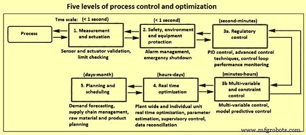
图5五个层次的过程控制和优化

一般而言，各种级别的控制应用都针对以下一个或多个目标，即 (i) 确定并维持过程在实际的最佳操作点，(ii) 维持安全操作以保护人员和设备，(iii) ) 最大限度地减少对操作员关注和干预的需求，以及 (iv) 最大限度地减少干扰和干扰的数量、程度和传播。

仪器 – 它由控制船尾的组件组成。仪表提供流程和控制层次之间的直接接口，是流程状态信息的基本来源，也是将纠正措施传输到流程的最终手段。过程测量设备的功能是感测过程变量的值或值的变化。实际的传感设备可以产生物理运动、压力信号和毫伏信号等。传感器将测量信号从一种物理或化学量转换为另一种，例如压力转换为毫安。然后将转换后的信号通过传输线传输到控制室。因此，发射器是一个信号发生器和一个线路驱动器。现代控制设备需要数字信号用于显示和控制算法，因此模数转换器（ADC）将变送器的模拟信号转换为数字格式。

最常测量的过程变量是温度、流量、压力、液位和成分。适当时，还测量其他物理特性。为特定应用选择合适的仪器取决于以下因素，例如所涉及的流体或固体的类型和性质、相关的工艺条件、所需的范围、精度和可重复性、响应时间、安装成本以及可维护性和可靠性。

信号传输和调理 – 各种各样的现象用于测量表征过程状态所需的过程变量。因为大多数过程都是在控制室中操作的，所以这些值在那里是可用的。 Hence, the measurements are usually transduced to an electronic form, most often 4-20 mA, and then transmitted to a remote terminal unit and then to the control room. It is especially important that proper care is taken so that these measurement signals are not corrupted owing to ground currents, interference from other electrical equipment and distribution, and other sources of noise.

Final control elements – Good control at any hierarchial level needs good performance by the final control elements in the next lower level. At the higher control levels, the final control element can be a control application at the next lower control level. However, the control command ultimately affects the process through the final control elements at the regulatory control level, e.g., control valves, pumps, dampers, louvers, and feeders etc.

Process dynamics and mathematical models – A thorough understanding of the time-dependent behaviour of the technological processes is required in order to instrument and control the process. This in turn requires an appreciation of how mathematical tools can be employed in analysis and design of process control systems. There are several mathematical principles which are utilized for the automatic control. These are (i) physical models and empirical models, (ii) simulation of dynamic models, (iii) Laplace transforms, transfer functions, and block diagrams, and (iv) fitting dynamic models to experimental data etc.

Feed -back control systems – Measurements of the controlled variable are available in many process control problems. Specifically, this is the case when temperatures, pressure, or flows are to be controlled. In these situations the controlled variable can be directly measured and the manipulated variable is adjusted via a final control element. A feedback controller takes action when the controlled variable deviates from its set-point, as detected by the non-zero value of the error signal. The various types of feed-back controls are (i) on/off control, (ii) proportional control, (iii) proportional plus integral (PI) control, (iv) proportional plus integral plus derivative (PID) control, and (v) digital PID.

The simplest controller can only show two settings and is called an on/off controller. The output of this controller is either at its maximum or its minimum value, depending on the sign of the error. While this type of controller is simple, it is seldom used.  The proportional controller offers more flexibility than the on/off controller because the manipulated variable is related not just to the sign of the error but also to its magnitude. The input-output behaviour of an actual proportional controller has upper and lower bounds i.e. the output saturates when the control limits are reached. Standard limits on the controller output are 3-15 PSI for pneumatic controllers, 4-20mA for electric controllers, and 0-10 VDC for digital controllers.

Integrating action needs to be included in the control loop, if an offset-free response in the presence of constant load disturbances or for set point changes is needed. If the process does not show integrating behaviour itself then it is possible to implement a proportional plus-integral controller to achieve the desired performance. There are both and disadvantages associated with integral action in a controller. One disadvantage of a PI controller is that the integral action can cause it to react more sluggishly than a proportional controller. If it is important to achieve a faster response which is to be offset-free then this can be accomplished by including both derivative and integral action in the controller. In order to anticipate the future behaviour of the error signal, a PID controller computes the rate of change of the error, thus the directional trend of the error signal influences the controller output. While many controllers have traditionally been analog PI/PID controllers, the trend towards digital control systems has also had an influence on controller implementation. In many modern process plants the analog PI/PID controllers have been replaced by the digital counterparts.

Open-loop and closed-loop dynamics – Open-loop dynamics refers to the behaviour of a process if no controller is acting on it. Similarly, if the controller is turned off by setting the proportional constant to zero, the control system shows open-loop behaviour and the system’s dynamics are solely determined by the process. Hence, it is not possible to reach a new set-point for a process in open-loop unless the input is changed manually. It is also not possible to reject disturbances when the process is operated without a controller.

The purpose of using closed-loop control is to achieve a desired performance for the system. This can result in the system being stabilized, in a faster system response to the set-point changes, or in the ability to reject disturbances. The choice of the controller type as well as the values of the controller tuning parameters influences the closed-loop behaviour. For a controlled process one needs to find controller settings which result in a fast system response with little or no offset. At the same time, the system is to be robust to the changes in process characteristics. Finding the appropriate settings is called ‘tuning’ the controller.

Controller tuning and stability – Finding of the optimum tuning parameters for a controller is an important task. Unsuitable parameters can result in not achieving the desired closed-loop performance (e.g. slowly decaying oscillations, or a slow acting process). It is also possible that a closed-loop process with a badly tuned controller can result in performance which is worse than for the open-loop case or that the process can even become unstable.

Mathematical software for process control – A variety of different software packages is available which support the controller design, controller testing, and implementation process.

Advanced control techniques

While the single-loop PI/PID feedback controller is satisfactory for many process applications, there are cases for which advanced control techniques can result in a significant improvement in closed-loop performance. These processes often show one or more of such phenomena as (i) slow dynamics, (ii) time delays, (iii) frequent disturbances, (iv) multi-variable interaction. A large number of advanced control strategies are being used. Some important ones are briefly discussed below.

Feed- forward control – One of the disadvantages of conventional feed-back control with large time lags or delays is that disturbances are not recognized until after the controlled variable deviates from its set point. However, if it is possible to measure the load disturbance directly then feed-forward control can be applied in order to minimize the effect which this load disturbance has on the controlled variable. In addition to being able to measure the load disturbance, it is also needed to determine a mathematical correlation for the effect which the load disturbance has on the controlled variable in order to apply a feed-forward controller. The reason for this is that the feed-forward controller inverts this model in order to cancel the effect that the disturbance has. A feed-forward controller can be designed either based on the steady-state or dynamic behavior of the process.

Cascade control – Another possibility of controlling processes with multiple or slow-acting disturbances, is to implement cascade control. The main idea behind cascade control is that more than just one controller is used to reject disturbances. Instead a secondary controller is added to take action before the slow-acting disturbance has an effect on the primary controlled variable. In order to achieve this, the secondary controller also requires a secondary measurement point which needs to be located so that it recognizes the upset condition before the primary controlled variable is affected. Cascade control strategies are among the most popular process control strategies.

Selective and override control – Some processes have more controlled variables than manipulated variables. Such a situation does not allow an exact pairing of controlled and manipulated variables. A common solution is to use a device called a selector which chooses the appropriate process variable from among a number of valid measurements. The purpose of the selector is to improve control system performance as well as to protect equipment from unsafe operating conditions by choosing appropriate controlled variables for a specific process operating condition. Selectors can be based on multiple measurement points, multiple final control elements, or multiple controllers.

Adaptive control and auto-tuning – Operating conditions of a process can frequently change during plant operations. This does lead to the process behaving differently from the model which has been used for the controller design. Hence, the controller does not have accurate knowledge of the process at the current operating point and hence cannot be able to provide adequate disturbance rejection or set-point tracking. One possibility to circumvent this is to use an adaptive control system which automatically adjusts the controller parameters to compensate for changing process conditions. Auto-tuning is a related method where the closed-loop system is periodically tested, and the test characteristics automatically determine new controller settings.

Fuzzy logic control – For many processes, it is very time consuming to determine accurate process models. However, at the same time, it can be intuitive to get a rough estimate of how the manipulated variable is to react to a process condition. For such a case, fuzzy logic controllers can offer an advantage over conventional PID controllers. The reason for this is that fuzzy controllers do not need an exact mathematical description of a process. Instead, they classify the controller inputs and output as belonging to one of several groups (i.e. low, normal, and high). Fuzzy rules are then used to compute the output category from the given inputs. These rules either have to be provided by the control engineer or they have to be identified from plant operations by auto-tuning. It is also possible to combine fuzzy logic controllers with neural networks in order to form neuro-fuzzy controllers. This type of controller can offer significant advantages over conventional PID when applied to non-linear systems whose characteristics change over time.

Statistical process control (SPC) – SPC, also called statistical quality control (SQC), has found widespread application in recent years due to the growing focus on increased productivity. Another reason for its increasing use is that feed-back control cannot be applied to many processes due to a lack of on-line measurements. However, it is important to know if these processes are operating satisfactorily. While SPC is unable to take corrective action while the process is moving away from the desired target, it can serve as an indicator that product quality might not be satisfactory and that corrective action are to be taken for further plant operations.

For a process which is operating satisfactorily, the variation of product quality falls within acceptable limits. These limits normally correspond to the minimum and maximum values of a specified property. Normal operating data can be used to compute the mean deviation and the standard deviation s of a given process variable from a series of observations. The standard deviation is a measure for how the values of the variable spread around the mean. A large value indicates that wide variations in the variable. Assuming the process variable follows a normal probability distribution, then 99.7 % of all observations is to lie within an upper limit and a lower limit. This can be used to determine the quality of the control. If all data from a process lie within the limits, then it can be concluded that nothing unusual has happened during the recorded time period, the process environment is relatively unchanged, and the product quality lies within specifications. On the other hand, if repeated violations of the limits occur, then the conclusion can be drawn that the process is out of control and that the process environment has changed. Once this has been determined, the process operator can take action in order to adjust operating conditions to counteract undesired changes which have occurred in the process conditions.

Multi-variable control – Many technological processes contain several manipulated as well as controlled variables. These processes are called multi-variable control systems. It is possible to analyze the interactions among the control loops with techniques like the relative gain array. If it turns out that there are only small interactions between the loops then it is possible to pair the inputs and outputs in a favourable way and use single loop controllers which can be tuned independently from one another. However, if strong interactions exist, then the controllers need to be detuned in order to reduce oscillations.

Model predictive control (MPC) – MPC is a model-based control technique. It is the most popular technique for handling multi-variable control problems with multiple inputs and multiple outputs (MIMO) and can also accommodate inequality constraints on the inputs or outputs such as upper and lower limits. All of these problems are addressed by MPC by solving an optimization problem and therefore no complicated override control strategy is needed. A variety of different types of models can be used for the prediction. Choosing an appropriate model type is dependent upon the application to be controlled. The model can be based upon first-principles or it can be an empirical model. Also, the supplied model can be either linear or nonlinear, as long as the model predictive control software supports this type of model.

Real-time optimization – Operating objectives for process facilities are set by economics, product orders, availability of raw materials and utilities, etc. At different points in time it can be advantageous or necessary to operate a process in different ways to meet a particular operating objective. A technological process, however, is a dynamic, integrated environment where external and internal conditions can cause the optimal operating point for each operating objective to vary from time to time. These operating points can be computed by real-time process optimization (RTO), where the optimization can be performed on several levels, ranging from optimization within model predictive controllers, to supervisory controllers which determine the targets for optimum operation of the process, to optimization of production cycles. The plant-wide problems which can be solved by optimization techniques on a daily or hourly basis can be large containing thousands or even tens of thousands of variables.

Batch and sequence control

In batch processes, the product is made in discrete batches by sequentially performing a number of processing steps in a defined order on the raw materials and intermediate products. Large production runs are achieved by repeating the process. The term recipe has a range of definitions in batch processing, but in general a recipe is a procedure with the set of data, operations, and control steps to manufacture a particular grade of product. A formula is the list of recipe parameters, which includes the raw materials, processing parameters, and product outputs. A recipe procedure has operations for both normal and abnormal conditions. Each operation contains resource requests for certain ingredients (and their amounts). The operations in the recipe can adjust set-points and turn equipment on and off. The complete production run for a specific recipe is called a campaign (multiple batches). A production run consists of a specified number of batches using the same raw materials and making the same product to satisfy customer demand. The accumulated batches are called a lot.

In multi-grade batch processing, the instructions remain the same from batch to batch, but the formula can be changed to yield modest variations in the product. In flexible batch processing, both the formula (recipe parameters) and the processing instructions can change from batch to batch. The recipe for each product must specify both the raw materials required and how conditions within the reactor are to be sequenced in order to make the desired product.

Batch process control hierarchy – Functional control activities for batch process control can be summarized in four categories namely (i) batch sequencing and logic control, (ii) control during the batch, (iii) run-to- run control, and (iv) batch production management.

In batch sequencing and logic control, sequencing of control steps follow the recipe involve. For example:mixing of ingredients, heating, waiting for a reaction to complete, cooling, or discharging the resulting product. Transfer of materials to and from batch reactors includes metering of materials as they are charged (as specified by each recipe), as well as transfer of materials at the completion of the process operation. In addition to discrete logic for the control steps, logic is needed for safety interlocks to protect personnel, equipment, and the environment from unsafe conditions. Process interlocks ensure that process operations can only occur in the correct time sequence for a prescribed period of time. Detection of when the batch operations are to be terminated (end point) can be performed by inferential measurements of product quality, if direct measurement is not feasible.

Run-to-run control (also called batch-to-batch) is a supervisory function based on off-line product quality measurements at the end of a run. Operating conditions and profiles for the batch are adjusted between runs to improve the product quality using tools such as optimization. Batch production management entails advising the plant operator of process status and how to interact with the recipes and the sequential, regulatory, and discrete controls. Complete information (recipes) is maintained for manufacturing each product grade, including the names and amounts of ingredients, process variable set points, ramp rates, processing times, and sampling procedures. Other database information includes batches produced on a shift, daily, or weekly basis, as well as material and energy balances. Scheduling of process units is based on availability of raw materials and equipment and customer demand.

Sequential function charts – Compared to a continuous process, batch process control requires a greater percentage of discrete logic and sequential control than regulatory control loops. Batch control applications is to control the timing and sequencing of the process steps based on discrete input and outputs as well as analog outputs. The complexity of the interactive logic within and between the various control levels, the required interactions with operators and the need for ongoing application modification and maintenance are reasons why organization, functional design, and clear documentation are so important to the successful use of batch control applications. In order to describe what is to be done, structural models are normally used to represent the required batch processing actions, the batch equipment, and the combination of components. Various formats have been proposed for describing the batch control applications, e.g., how the batch processing steps are carried out with the batch equipment and instrumentation, interfaces between the various levels of control, interfaces between the batch control and the operator actions and responses, and interactions and coordination with the safety interlocks. The formats proposed include flow charts, state charts, decision tables, structured pseudo-code, state transition diagrams, petri nets, and sequential function charts. A sequential function chart (SFC) describes graphically the sequential behaviour of a control program.