一种基于纳米天线粒子的智能给药系统的新设计

摘要

复合纳米颗粒给药系统在与淋巴结的相互作用中起着重要作用。淋巴细胞主要分为三种类型：B 细胞、T 细胞和自然杀伤细胞。当免疫系统的细胞致癌时，它们会攻击身体细胞。淋巴液在攻击身体健康细胞方面起着重要作用；因此，本文旨在设计一种药物递送系统，该系统可以有效地引导纳米粒子靶向受感染的细胞，从而帮助高速消除此类细胞。所提出的设计取决于这些分子之间的相互作用，智能纳米控制器具有通过厌氧接触引导纳米颗粒的能力。所提出的设计证明，纳米颗粒的尺寸和密度越小，液体的动态粘度就越小，这将反映其流动阻力。此外，还得出结论，氢分子由于其密度低而在降低淋巴液阻力方面发挥着重要作用。

介绍

目前的癌症治疗选择包括手术、放疗和化疗。这些治疗策略也会伤害普通组织并导致恶性生长的部分消灭。因此，纳米技术可以通过专门针对有害细胞和肿瘤、直接切除肿瘤以及提高基于辐射和其他治疗方式的有效性来克服这些缺点。这可以显着减少治疗的副作用并提高存活率。纳米技术是治疗恶性生长的一种很有前途的工具，因为它通过使用纳米材料提供更新和更好的治疗方式。纳米粒子可以特异性靶向癌细胞上差异表达的许多分子。纳米粒子的通常广阔的翼型区域可以用配体例如小粒子和脱氧核糖核酸腐蚀性或核糖核酸腐蚀性链肽抗体进行功能化。配体用作药物和治疗诊断应用。纳米粒子的物理特性，如活力分散和再辐射，同样可用于影响患病组织，如激光去除和热疗应用[1]。

创新的纳米粒子软件程序和活性药物元素也将有助于探索更广泛的活性成分。因此，正在研究免疫原性货物和表面涂层作为纳米颗粒介导的和传统化学疗法的佐剂。这一创新策略包括将纳米颗粒设计为呈现在细胞上的人工抗原和发挥抗肿瘤作用的刺激因子的体内储存库。纳米技术代表了具有许多应用的活跃研究领域。纳米颗粒由于其可调节的物理化学特性，如解冻指数点、亲水性、导电和导热、催化活性、光吸收和散射，在医疗技术中引起了人们的兴趣 [2]。原则上，纳米材料被描述为颗粒在 1 到 100 nm 范围内的材料。欧盟和美国有几项立法专门针对使用纳米材料的医学研究。然而，对于纳米材料，国际上并没有公认的定义。不同的组织考虑不同的纳米材料概念 [3]。纳米颗粒药物递送系统的目标之一是用癌细胞治疗淋巴液。与淋巴结相互作用的复合纳米颗粒给药系统如图1所示。

<图片>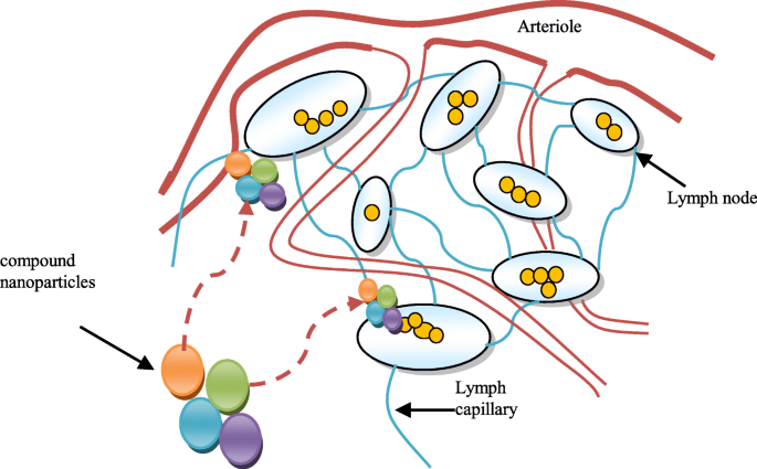

复合纳米颗粒给药系统及其与淋巴结的相互作用

美国食品和药物管理局将纳米材料称为颗粒在 1 到 100 范围内的材料，其特性不同于大块材料 [4, 5]。纳米纤维、纳米板、纳米线、量子点和其他相关材料已被表征 [6]。固体脂质纳米粒（SLNs）是一种脂质纳米粒（LN），可以利用固体脂质来构建[7]。已经开发了 SLN 的后续版本，例如纳米结构脂质载体 (NLC)，它们代表了 LN 的第二个时代 [8]。 SLN 和 NLC 都是由固体脂质构成的。 SLN 的内部结构包含固体脂质，而 NLC 是利用固体和液体脂质的混合物开发的，产生宝石横截面 [9, 10]。鉴于包含许多固体脂质片段的 SLN 可用于医疗应用 [11, 12] 的事实，还报告了 SLN 的这些缺陷。聚合物纳米粒子 (PN) 可以由天然聚合物或无机材料制成，例如二氧化硅 [13]。聚合物或脂质塑造了 NPs 的核心，提高了稳定性和药物输送，并提供了统一的形状和大小 [14]。 PN 可被描述为纳米胶囊或纳米球。纳米胶囊在囊泡结构中含有油和药物 [15, 16]，而纳米球含有不含油的聚合物链 [17, 18]。通过与聚合物混合，药物被包装在 PNs 中。在聚合时确保药物掺入纳米颗粒中。通过将药物溶解、散射或人工吸附在聚合物网络的成分中，PNs 加载了药物 [19, 20]。淋巴细胞分为三种类型：B 细胞、T 细胞和自然杀伤细胞。 B 细胞产生抗体来攻击入侵的微生物，而当它们变得致癌时，它们也会攻击免疫系统。因此，考虑到淋巴液在自身免疫中的重要作用，本文的目的是设计一种基于纳米天线颗粒的智能给药系统。因此，该系统包含许多不同数量的纳米粒子。下一节介绍智能给药系统的设计。

纳米智能给药系统的设计

所提出的纳米智能药物输送系统包含一个由纳米压电材料制成的纳米粒子电源操作的纳米控制器。纳米粒子的复杂储存库有许多微型储存库。每个小型存储库都包含一种类型的纳米粒子。纳米粒子分子包含一个设计用于与纳米控制器通信的纳米天线。拟议的纳米智能药物输送系统还包含碳纳米管，用于将药物快速输送到癌细胞。它可以与受感染的细胞相关联，如图 2 所示。该系统首先将纳米粒子发送到称为“探索性纳米粒子”的癌细胞。这些分子通过厌氧通讯将它们在细胞内的位置的完整图片发送到纳米控制器。根据探索性纳米粒子遇到的情况，纳米控制器根据从探索性纳米粒子收集的信息，向癌细胞发送不同数量、类型和密度的纳米粒子。这些纳米粒子被称为“战斗纳米粒子”。

<图片>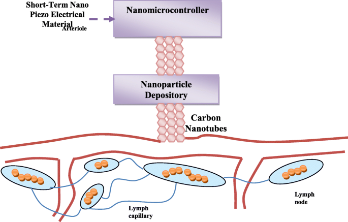

显示所提出的药物系统与受感染细胞的关联的一般结构

这不是随机过程，而是由纳米控制器考虑多个方面和对数进行控制，这将确保纳米颗粒的高效和快速输送。为了准确快速地将纳米颗粒输送到癌细胞，将采用压缩二进制搜索算法 [21]。此外，纳米颗粒将以不同的密度输送，从而使药物变得更有效。这些方法及其使用纳米控制器的方法如图 3 所示。纳米控制器的物理结构类似于纳米颗粒，但它是金属的形式，因此可以获得电能工作期间的一小段时间。这种金属包含一个无线天线和一个小存储器，其中包含操作代码，纳米控制器和纳米粒子商店之间有纳米粒子链接。纳米粒子存储库包含几种不同类型的纳米粒子。将控制纳米门的打开和关闭以及打开的持续时间，以定制要输送的粒子数量。

<图片>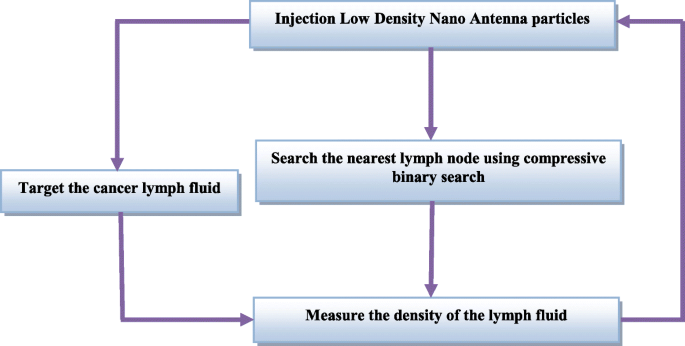

抗击纳米粒子向癌细胞的发送过程

对拟议药物系统中使用的纳米颗粒性质的描述

在下一节中，将讨论在提议的药物递送系统中使用的纳米粒子的性质。在这项工作中，使用了低密度厌氧纳米粒子，如早期报告中所述[22]。

低密度纳米粒子

将用于癌症的复合纳米颗粒的药物递送过程视为淋巴液中的穿透过程，其中肿瘤被淋巴液包围。黑色素瘤的成分类似于淋巴液。所提出的分析模型基于由三种不同类型的纳米粒子组成的纳米管系统。纳米颗粒被放置在高密度淋巴液中。我们可以将球形极坐标中固体 A 的特定纳米粒子定义为 A =(ra, ϑa , φa)，其中 ra 是固体 A 的纳米粒子的径向坐标，ϑa 是固体A纳米粒子的天顶坐标，φa是固体A纳米粒子的方位坐标。固体B对应的坐标是B 分别为 =(rb, ϑb, φb)，对应的立体 N 坐标为 N 分别为 =(rn, ϑn, φn)。考虑到淋巴结有两个特性，即触痛和肿胀，它们受到霍奇金淋巴瘤癌细胞的影响。具有触痛性 Tp 的淋巴结可描述为 Tp (N ,t );这意味着与固体 N 纳米粒子流体相关的 Tp 值随时间变化。现在，让我们考虑复合纳米粒子对柔韧性的总影响定义为：

$$ \mathrm{Tpt}=\mathrm{Tp}\ \left(A,t\right)+\mathrm{Tp}\ \left(B,t\right)+.\dots \dots \dots \dots + \mathrm{Tp}\ \left(N,t\right) $$ (1)

考虑膨胀属性的相同情况，它可以定义为：

$$ \mathrm{Tst}=\mathrm{Ts}\ \left(A,t\right)+\mathrm{Ts}\ \left(B,t\right)+.\dots \dots \dots \dots + \mathrm{Ts}\ \left(N,t\right) $$ (2)

从方程。由 1 和 2 可知，这两种性质随时间的变化率可以确定为：

$$ \frac{\partial \left(\mathrm{Tp}\left(A,t\right)\right)}{\partial t}+\frac{\partial \left(\mathrm{Tp}\left( B,t\right)\right)}{\partial t}+\dots \frac{\partial \left(\mathrm{Tp}\left(N,t\right)\right)}{\partial t}=\frac{\mathrm{\partial Tp}(t)}{\mathrm{\partial t}} $$ (3) $$ \frac{\partial \left(\mathrm{Ts}\left(A,t\ right)\right)}{\partial t}+\frac{\partial \left(\mathrm{Ts}\left(B,t\right)\right)}{\partial t}+\dots \frac{\部分 \left(\mathrm{Ts}\left(N,t\right)\right)}{\partial t}=\frac{\mathrm{\partial Ts}(t)}{\partial t} $$ ( 4)

淋巴液中一个纳米固体 N 颗粒所能占据的点定义为：

$$ {\mathrm{Po}}_n=\mathrm{Po}{\left(\mathrm{po},t\right)}_n $$ (5)

让我们考虑一个柔软淋巴液的固体 N 衍生物的纳米颗粒被定义为 $ \frac{\partial {\left(\mathrm{Tp}\left(N,t\right)\right)}_{\ mathrm{po}}}{\partial t} $，那么嫩淋巴液的复合材料导数将等于：

$$ \frac{\partial {\left(\mathrm{Tp}\left(A,t\right)\right)}_{\mathrm{po}}}{\partial t}+\frac{\partial { \left(\mathrm{Tp}\left(B,t\right)\right)}_{\mathrm{po}}}{\partial t}+\dots \frac{\partial {\left(\mathrm{ Tp}\left(N,t\right)\right)}_{\mathrm{po}}}{\partial t}=\frac{\mathrm{\partial Tp}{(t)}_{\mathrm{ po}}}{\partial t} $$ (6) $$ \frac{\partial {\left(\mathrm{Ts}\left(A,t\right)\right)}_{\mathrm{po} }}{\partial t}+\frac{\partial {\left(\mathrm{Ts}\left(B,t\right)\right)}_{\mathrm{po}}}{\partial t}+ \dots \frac{\partial {\left(\mathrm{Ts}\left(N,t\right)\right)}_{\mathrm{po}}}{\partial t}=\frac{\mathrm{ \partial Ts}{(t)}_{\mathrm{po}}}{\partial t} $$ (7)

固体 N 的相应速度分量取为 (v rn, v ϑn, v φn)。然后，在淋巴液的动态粘度 dν 和 p 下，固体 N 粒子的流速使用纳维-斯托克斯方程表示是压力和 ρ 是淋巴液的密度如下：

$$ \frac{\partial {v}_{\mathrm{rn}}}{\partial t}+{v}_{\mathrm{rn}}\frac{\partial {v}_{\mathrm{rn }}}{\mathrm{\partial rn}}+\frac{v_{\upvartheta \mathrm{n}}}{\mathrm{rn}}\frac{\partial {v}_{\mathrm{rn}} }{\mathrm{\partial \upvartheta n}}+\frac{v_{\upvarphi \mathrm{n}}}{\mathrm{rn}\ \mathrm{sin}\upvartheta \mathrm{n}}\frac{ \partial {v}_{\mathrm{rn}}}{\mathrm{\partial \upvarphi n}}-\frac{v_{\upvartheta \mathrm{n}}^2}{\mathrm{rn}}- \frac{v_{\upvarphi \mathrm{n}}^2}{\mathrm{rn}}+\frac{1}{\rho}\frac{\partial p}{\mathrm{\partial rn}}- \mathrm{d}\upnu \left[\frac{1}{{\mathrm{rn}}^2}\frac{\partial }{\mathrm{\partial rn}}\left({\mathrm{rn} }^2\frac{\partial {v}_{\mathrm{rn}}}{\mathrm{\partial rn}}\right)+\frac{1}{{\mathrm{rn}}^2\mathrm {sin}\upvartheta \mathrm{n}}\frac{\partial }{\mathrm{\partial \upvartheta n}}\left(\mathrm{sin}\upvartheta \mathrm{n}\frac{\partial {v }_{\mathrm{rn}}}{\mathrm{\partial \upvartheta n}}\right)+\frac{1}{{\mathrm{rn}}^2{\sin}^2\upvartheta \mathrm {n}}\frac{\partial^2{v}_{\ma thrm{rn}}}{\partial {\upvarphi \mathrm{n}}^2}+-\frac{2{v}_{\mathrm{rn}}}{{\mathrm{rn}}^2} -\frac{2}{{\mathrm{rn}}^2\sin \upvartheta \mathrm{n}}\frac{\partial \left({v}_{\upvartheta \mathrm{n}}\mathrm{ sin}\upvartheta \mathrm{n}\right)}{\mathrm{\partial \upvartheta n}}-\frac{2}{{\mathrm{rn}}^2\mathrm{sin}\upvartheta \mathrm{ n}}\frac{\partial {v}_{\upvarphi \mathrm{n}}}{\partial_{\upvarphi \mathrm{n}}}\right]=0 $$ (8)

淋巴液的动力粘度dν计算如下：

固体 A 和 B 的纳维-斯托克斯方程可以表示为方程。 8 和 9。因此，方程。 9 可以表示为：

$$ \mathrm{d}\upnu =\frac{\left[\frac{\partial {v}_{\mathrm{rn}}}{\partial t}+{v}_{\mathrm{rn}} \frac{\partial {v}_{\mathrm{rn}}}{\mathrm{\partial rn}}+\frac{v_{\upvartheta \mathrm{n}}}{\mathrm{rn}}\frac {\partial {v}_{\mathrm{rn}}}{\mathrm{\partial \upvartheta n}}+\frac{v_{\upvarphi \mathrm{n}}}{\mathrm{rn}\ \mathrm {sin}\upvartheta \mathrm{n}}\frac{\partial {v}_{\mathrm{rn}}}{\mathrm{\partial \upvarphi n}}-\frac{v_{\upvartheta \mathrm{ n}}^2}{\mathrm{rn}}-\frac{v_{\upvarphi \mathrm{n}}^2}{\mathrm{rn}}+\frac{1}{\rho}\frac{ \partial p}{\mathrm{\partial rn}}\right]}{\left[\frac{1}{{\mathrm{rn}}^2}\frac{\partial }{\mathrm{\partial rn }}\left({\mathrm{rn}}^2\frac{\partial {v}_{\mathrm{rn}}}{\mathrm{\partial rn}}\right)+\frac{1}{ {\mathrm{rn}}^2\mathrm{sin}\upvartheta \mathrm{n}}\frac{\partial }{\mathrm{\partial \upvartheta n}}\left(\mathrm{sin}\upvartheta \ mathrm{n}\frac{\partial {\mathrm{v}}_{\mathrm{rn}}}{\mathrm{\partial \upvartheta n}}\right)+\frac{1}{{\mathrm{ rn}}^2{\sin}^2\upvartheta \math rm{n}}\frac{\partial^2{\mathrm{v}}_{\mathrm{rn}}}{\partial {\upvarphi \mathrm{n}}^2}-\frac{2{\ mathrm{v}}_{\mathrm{rn}}}{{\mathrm{rn}}^2}-\frac{2}{{\mathrm{rn}}^2\sin \upvartheta \mathrm{n} }\frac{\partial \left({\mathrm{v}}_{\upvartheta \mathrm{n}}\mathrm{sin}\upvartheta \mathrm{n}\right)}{\mathrm{\partial \upvartheta n}}-\frac{2}{{\mathrm{rn}}^2\mathrm{sin}\upvartheta \mathrm{n}}\frac{\partial {\mathrm{v}}_{\upvarphi \mathrm {n}}}{\partial_{\upvarphi \mathrm{n}}}\right]}=\frac{\left[\frac{\partial {\mathrm{v}}_{\mathrm{ra}}} {\mathrm{\partial t}}+{\mathrm{v}}_{\mathrm{ra}}\frac{\partial {\mathrm{v}}_{\mathrm{ra}}}{\mathrm{ \partial ra}}+\frac{{\mathrm{v}}_{\upvartheta \mathrm{a}}}{\mathrm{ra}}\frac{\partial {\mathrm{v}}_{\mathrm {ra}}}{\mathrm{\partial \upvartheta a}}+\frac{{\mathrm{v}}_{\upvarphi \mathrm{a}}}{\mathrm{ra}\ \mathrm{sin} \upvartheta \mathrm{a}}\frac{\partial {\mathrm{v}}_{\mathrm{ra}}}{\mathrm{\partial \upvarphi a}}-\frac{{\mathrm{v} }_{\upvartheta \mathrm{a}}^2}{\mathrm{ra}}- \frac{{\mathrm{v}}_{\upvarphi \mathrm{a}}^2}{\mathrm{ra}}+\frac{1}{\uprho}\frac{\mathrm{\partial p} }{\mathrm{\partial ra}}\right]}{\left[\frac{1}{{\mathrm{ra}}^2}\frac{\partial }{\mathrm{\partial ra}}\ left({\mathrm{ra}}^2\frac{\partial {v}_{\mathrm{ra}}}{\mathrm{\partial ra}}\right)+\frac{1}{{\mathrm {ra}}^2\mathrm{sin}\upvartheta \mathrm{a}}\frac{\partial }{\mathrm{\partial \upvartheta a}}\left(\mathrm{sin}\upvartheta \mathrm{a }\frac{\partial {v}_{\mathrm{ra}}}{\mathrm{\partial \upvartheta a}}\right)+\frac{1}{{\mathrm{ra}}^2{\ sin}^2\upvartheta \mathrm{a}}\frac{\partial^2{v}_{\mathrm{ra}}}{\partial {\upvarphi \mathrm{a}}^2}-\frac{ 2{v}_{\mathrm{ra}}}{{\mathrm{ra}}^2}-\frac{2}{{\mathrm{ra}}^2\sin \upvartheta \mathrm{a}} \frac{\partial \left({v}_{\upvartheta \mathrm{a}}\mathrm{sin}\upvartheta \mathrm{a}\right)}{\mathrm{\partial \upvartheta a}}-\压裂{2}{{\mathrm{ra}}^2\mathrm{sin}\upvartheta \mathrm{a}}\frac{\partial {v}_{\upvarphi \mathrm{a}}}{\partial_{ \upvarphi \mathrm{a}}}\right]}=\frac{ \left[\frac{\partial {v}_{\mathrm{rb}}}{\partial t}+{v}_{\mathrm{rb}}\frac{\partial {v}_{\mathrm{ rb}}}{\mathrm{\partial rb}}+\frac{v_{\upvartheta \mathrm{b}}}{\mathrm{rb}}\frac{\partial {v}_{\mathrm{rb} }}{\mathrm{\partial \upvartheta b}}+\frac{v_{\upvarphi \mathrm{b}}}{\mathrm{rb}\ \mathrm{sin}\upvartheta \mathrm{b}}\frac {\partial {v}_{\mathrm{rb}}}{\mathrm{\partial \upvarphi b}}-\frac{v_{\upvartheta \mathrm{b}}^2}{\mathrm{rb}} -\frac{v_{\upvarphi \mathrm{b}}^2}{\mathrm{rb}}+\frac{1}{\rho}\frac{\partial p}{\mathrm{\partial rb}} \right]}{\left[\frac{1}{{\mathrm{rb}}^2}\frac{\partial }{\mathrm{\partial rb}}\left({\mathrm{rb}}^ 2\frac{\partial {v}_{\mathrm{rb}}}{\mathrm{\partial rb}}\right)+\frac{1}{{\mathrm{rb}}^2\mathrm{sin }\upvartheta \mathrm{b}}\frac{\partial }{\mathrm{\partial \upvartheta b}}\left(\mathrm{sin}\upvartheta \mathrm{b}\frac{\partial {v}_ {\mathrm{rb}}}{\mathrm{\partial \upvartheta b}}\right)+\frac{1}{{\mathrm{rb}}^2{\sin}^2\upvartheta \mathrm{b }}\frac{\partial^2{v}_{\mathrm{ rb}}}{\partial {\upvarphi \mathrm{b}}^2}-\frac{2{v}_{\mathrm{rb}}}{{\mathrm{rb}}^2}-\frac {2}{{\mathrm{rb}}^2\sin \upvartheta \mathrm{b}}\frac{\partial \left({v}_{\upvartheta \mathrm{b}}\mathrm{sin}\ upvartheta \mathrm{b}\right)}{\mathrm{\partial \upvartheta b}}-\frac{2}{{\mathrm{rb}}^2\mathrm{sin}\upvartheta \mathrm{b}} \frac{\partial {v}_{\upvarphi \mathrm{b}}}{\partial_{\upvarphi \mathrm{b}}}\right]} $$ (10)

颗粒为纳米级；因此，它们的半径将非常小，为简单起见，方程。 10表示如下：

$$ \mathrm{d}\upnu =\left[\frac{v_{\upvartheta \mathrm{n}}}{\mathrm{rn}}\frac{\partial {v}_{\mathrm{rn}} }{\mathrm{\partial \upvartheta n}}+\frac{v_{\upvarphi \mathrm{n}}}{\mathrm{rn}\ \mathrm{sin}\upvartheta \mathrm{n}}\frac{ \partial {v}_{\mathrm{rn}}}{\mathrm{\partial \upvarphi n}}-\frac{v_{\upvartheta \mathrm{n}}^2}{\mathrm{rn}}- \frac{v_{\upvarphi \mathrm{n}}^2}{\mathrm{rn}}+\frac{1}{\rho}\frac{\partial p}{\mathrm{\partial rn}}\ right]/\left[\frac{1}{{\mathrm{rn}}^2}\frac{\partial }{\mathrm{\partial rn}}\left({\mathrm{rn}}^2\ frac{\partial {v}_{\mathrm{rn}}}{\mathrm{\partial rn}}\right)+\frac{1}{{\mathrm{rn}}^2\mathrm{sin}\ upvartheta \mathrm{n}}\frac{\partial }{\mathrm{\partial \upvartheta n}}\left(\mathrm{sin}\upvartheta \mathrm{n}\frac{\partial {\mathrm{v} }_{\mathrm{rn}}}{\mathrm{\partial \upvartheta n}}\right)+\frac{1}{{\mathrm{rn}}^2{\sin}^2\upvartheta \mathrm {n}}\frac{\partial^2{\mathrm{v}}_{\mathrm{rn}}}{\partial {\upvarphi \mathrm{n}}^2}-\frac{2{\mathrm {v}}_{\mathrm{rn}}}{{\math rm{rn}}^2}-\frac{2}{{\mathrm{rn}}^2\sin \upvartheta \mathrm{n}}\frac{\partial \left({\mathrm{v}}_ {\upvartheta \mathrm{n}}\mathrm{sin}\upvartheta \mathrm{n}\right)}{\mathrm{\partial \upvartheta n}}-\frac{2}{{\mathrm{rn}} ^2\mathrm{sin}\upvartheta \mathrm{n}}\frac{\partial {\mathrm{v}}_{\upvarphi \mathrm{n}}}{\partial_{\upvarphi \mathrm{n}} }\right]=\left[\frac{{\mathrm{v}}_{\upvartheta \mathrm{a}}}{\mathrm{ra}}\frac{\partial {\mathrm{v}}_{ \mathrm{ra}}}{\mathrm{\partial \upvartheta a}}+\frac{{\mathrm{v}}_{\upvarphi \mathrm{a}}}{\mathrm{ra}\ \mathrm{ sin}\upvartheta \mathrm{a}}\frac{\partial {\mathrm{v}}_{\mathrm{ra}}}{\mathrm{\partial \upvarphi a}}-\frac{{\mathrm{ v}}_{\upvartheta \mathrm{a}}^2}{\mathrm{ra}}-\frac{{\mathrm{v}}_{\upvarphi \mathrm{a}}^2}{\mathrm {ra}}+\frac{1}{\uprho}\frac{\mathrm{\partial p}}{\mathrm{\partial ra}}\right]/\left[\frac{1}{{\mathrm {ra}}^2}\frac{\partial }{\mathrm{\partial ra}}\left({\mathrm{ra}}^2\frac{\partial {\mathrm{v}}_{\mathrm {ra}}}{\mathrm{\partial ra}}\rig ht)+\frac{1}{{\mathrm{ra}}^2\mathrm{sin}\upvartheta \mathrm{a}}\frac{\partial }{\mathrm{\partial \upvartheta a}}\left (\mathrm{sin}\upvartheta \mathrm{a}\frac{\partial {\mathrm{v}}_{\mathrm{ra}}}{\mathrm{\partial \upvartheta a}}\right)+\压裂{1}{{\mathrm{ra}}^2{\sin}^2\upvartheta \mathrm{a}}\frac{\partial^2{\mathrm{v}}_{\mathrm{ra}} }{\partial {\upvarphi \mathrm{a}}^2}-\frac{2{\mathrm{v}}_{\mathrm{ra}}}{{\mathrm{ra}}^2}-\压裂{2}{{\mathrm{ra}}^2\sin \upvartheta \mathrm{a}}\frac{\partial \left({\mathrm{v}}_{\upvartheta \mathrm{a}}\ mathrm{sin}\upvartheta \mathrm{a}\right)}{\mathrm{\partial \upvartheta a}}-\frac{2}{{\mathrm{ra}}^2\mathrm{sin}\upvartheta \ mathrm{a}}\frac{\partial {v}_{\upvarphi \mathrm{a}}}{\partial_{\upvarphi \mathrm{a}}}\right]=\left[\frac{v_{\ upvartheta \mathrm{b}}}{\mathrm{rb}}\frac{\partial {v}_{\mathrm{rb}}}{\mathrm{\partial \upvartheta b}}+\frac{v_{\ upvarphi \mathrm{b}}}{\mathrm{rb}\ \mathrm{sin}\upvartheta \mathrm{b}}\frac{\partial {v}_{\mathrm{rb}}}{\mathrm{\部分的 \ upvarphi b}}-\frac{v_{\upvartheta \mathrm{b}}^2}{\mathrm{rb}}-\frac{v_{\upvarphi \mathrm{b}}^2}{\mathrm{rb }}+\frac{1}{\rho}\frac{\partial p}{\mathrm{\partial rb}}\right]/\left[\frac{1}{{\mathrm{rb}}^2 }\frac{\partial }{\mathrm{\partial rb}}\left({\mathrm{rb}}^2\frac{\partial {v}_{\mathrm{rb}}}{\mathrm{\部分 rb}}\right)+\frac{1}{{\mathrm{rb}}^2\mathrm{sin}\upvartheta \mathrm{b}}\frac{\partial }{\mathrm{\partial \upvartheta b}}\left(\mathrm{sin}\upvartheta \mathrm{b}\frac{\partial {v}_{\mathrm{rb}}}{\mathrm{\partial \upvartheta b}}\right)+ \frac{1}{{\mathrm{rb}}^2{\sin}^2\upvartheta \mathrm{b}}\frac{\partial^2{v}_{\mathrm{rb}}}{\部分 {\upvarphi \mathrm{b}}^2}-\frac{2{v}_{\mathrm{rb}}}{{\mathrm{rb}}^2}-\frac{2}{{\ mathrm{rb}}^2\sin \upvartheta \mathrm{b}}\frac{\partial \left({v}_{\upvartheta \mathrm{b}}\mathrm{sin}\upvartheta \mathrm{b} \right)}{\mathrm{\partial \upvartheta b}}-\frac{2}{{\mathrm{rb}}^2\mathrm{sin}\upvartheta \mathrm{b}}\frac{\partial { v}_{\upvarphi \mathrm{b}}}{\partial _{\upvarphi \mathrm{b}}}\right] $$ (11)

等式 11 可以表示如下：

$$ \mathrm{d}\upnu =\mathrm{rn}\left[{v}_{\upvartheta \mathrm{n}}\frac{\partial {v}_{\mathrm{rn}}}{\ mathrm{\partial \upvartheta n}}+\frac{v_{\upvarphi \mathrm{n}}}{\ \mathrm{sin}\upvartheta \mathrm{n}}\frac{\partial {v}_{\ mathrm{rn}}}{\mathrm{\partial \upvarphi n}}-{v}_{\upvartheta \mathrm{n}}^2-{v}_{\upvarphi \mathrm{n}}^2+ \frac{\mathrm{rn}}{\rho}\frac{\partial p}{\mathrm{\partial rn}}\right]/\left[\frac{\partial }{\mathrm{\partial rn} }\left({\mathrm{rn}}^2\frac{\partial {v}_{\mathrm{rn}}}{\mathrm{\partial rn}}\right)+\frac{1}{\ mathrm{sin}\upvartheta \mathrm{n}}\frac{\partial }{\mathrm{\partial \upvartheta n}}\left(\mathrm{sin}\upvartheta \mathrm{n}\frac{\partial { v}_{\mathrm{rn}}}{\mathrm{\partial \upvartheta n}}\right)+\frac{1}{\sin^2\upvartheta \mathrm{n}}\frac{\partial^ 2{v}_{\mathrm{rn}}}{\partial {\upvarphi \mathrm{n}}^2}-2{v}_{\mathrm{rn}}-\frac{2}{\sin \upvartheta \mathrm{n}}\frac{\partial \left({v}_{\upvartheta \mathrm{n}}\mathrm{sin}\upvartheta \mathrm{n}\right)}{\mathrm{\标准杆tial \upvartheta n}}-\frac{2}{\mathrm{sin}\upvartheta \mathrm{n}}\frac{\partial {v}_{\upvarphi \mathrm{n}}}{\partial_{\ upvarphi \mathrm{n}}}\right]=\mathrm{ra}\left[{v}_{\upvartheta \mathrm{a}}\frac{\partial {v}_{\mathrm{ra}}} {\mathrm{\partial \upvartheta a}}+\frac{v_{\upvarphi \mathrm{a}}}{\ \mathrm{sin}\upvartheta \mathrm{a}}\frac{\partial {v}_ {\mathrm{ra}}}{\mathrm{\partial \upvarphi a}}-{v}_{\upvartheta \mathrm{a}}^2-{v}_{\upvarphi \mathrm{a}}^ 2+\frac{\mathrm{ra}}{\rho}\frac{\partial p}{\mathrm{\partial ra}}\right]/\left[\frac{\partial }{\mathrm{\partial ra}}\left({\mathrm{ra}}^2\frac{\partial {v}_{\mathrm{ra}}}{\mathrm{\partial ra}}\right)+\frac{1} {\mathrm{sin}\upvartheta \mathrm{a}}\frac{\partial }{\mathrm{\partial \upvartheta a}}\left(\mathrm{sin}\upvartheta \mathrm{a}\frac{\部分 {v}_{\mathrm{ra}}}{\mathrm{\partial \upvartheta a}}\right)+\frac{1}{\sin^2\upvartheta \mathrm{a}}\frac{\ partial^2{v}_{\mathrm{ra}}}{\partial {\upvarphi \mathrm{a}}^2}-2{v}_{\mathrm{ra}}-\frac{2}{ \罪\upvartheta \mathrm{a}}\frac{\partial \left({v}_{\upvartheta \mathrm{a}}\mathrm{sin}\upvartheta \mathrm{a}\right)}{\mathrm{\部分 \upvartheta a}}-\frac{2}{\mathrm{sin}\upvartheta \mathrm{a}}\frac{\partial {v}_{\upvarphi \mathrm{a}}}{\partial_{\ upvarphi \mathrm{a}}}\right]=\mathrm{rb}\left[{v}_{\upvartheta \mathrm{b}}\frac{\partial {v}_{\mathrm{rb}}} {\mathrm{\partial \upvartheta b}}+\frac{v_{\upvarphi \mathrm{b}}}{\ \mathrm{sin}\upvartheta \mathrm{b}}\frac{\partial {v}_ {\mathrm{rb}}}{\mathrm{\partial \upvarphi b}}-{v}_{\upvartheta \mathrm{b}}^2-{v}_{\upvarphi \mathrm{b}}^ 2+\frac{\mathrm{rb}}{\rho}\frac{\partial p}{\mathrm{\partial rb}}\right]/\left[\frac{\partial }{\mathrm{\partial rb}}\left({\mathrm{rb}}^2\frac{\partial {v}_{\mathrm{rb}}}{\mathrm{\partial rb}}\right)+\frac{1} {\mathrm{sin}\upvartheta \mathrm{b}}\frac{\partial }{\mathrm{\partial \upvartheta b}}\left(\mathrm{sin}\upvartheta \mathrm{b}\frac{\部分 {v}_{\mathrm{rb}}}{\mathrm{\partial \upvartheta b}}\right)+\frac{1}{\si n^2\upvartheta \mathrm{b}}\frac{\partial^2{v}_{\mathrm{rb}}}{\partial {\upvarphi \mathrm{b}}^2}-2{v} _{\mathrm{rb}}-\frac{2}{\sin \upvartheta \mathrm{b}}\frac{\partial \left({v}_{\upvartheta \mathrm{b}}\mathrm{sin }\upvartheta \mathrm{b}\right)}{\mathrm{\partial \upvartheta b}}-\frac{2}{\mathrm{sin}\upvartheta \mathrm{b}}\frac{\partial {v }_{\upvarphi \mathrm{b}}}{\partial_{\upvarphi \mathrm{b}}}\right] $$ (12)

纳米粒子的半径与癌症引起的淋巴粘度之间存在直接关系。如果淋巴液变得过于静止和粘稠，就无法正常发挥其循环和清除毒素、帮助抗癌的功能。如果纳米颗粒较小，淋巴癌细胞很容易被杀死。为了描述复合纳米粒子总量的传输，我们使用连续性方程并假设固体A、B和N三个纳米粒子如下：

$$ \frac{1}{{\mathrm{ra}}^2}\frac{\partial }{\mathrm{\partial ra}}\left({\mathrm{ra}}^2{v}_{ \mathrm{ra}}\right)+\frac{1}{\mathrm{ra}\ \mathrm{sin}\upvartheta \mathrm{a}}\frac{\partial }{\mathrm{\partial \upvartheta a }}\left(\sin {\upvartheta \mathrm{v}}_{\upvartheta \mathrm{a}}\right)+\frac{1}{\mathrm{ra}\ \mathrm{sin}\upvartheta \ mathrm{a}}\frac{\partial {v}_{\upvarphi \mathrm{a}}}{\mathrm{\partial \upvarphi a}}+\frac{1}{{\mathrm{rb}}^ 2}\frac{\partial }{\mathrm{\partial rb}}\left({\mathrm{rb}}^2{v}_{\mathrm{rb}}\right)+\frac{1}{ \mathrm{rb}\ \mathrm{sin}\upvartheta \mathrm{b}}\frac{\partial }{\mathrm{\partial \upvartheta b}}\left(\sin {\upvartheta v}_{\upvartheta \mathrm{b}}\right)+\frac{1}{\mathrm{rb}\ \mathrm{sin}\upvartheta \mathrm{b}}\frac{\partial {v}_{\upvarphi \mathrm{ b}}}{\mathrm{\partial \upvarphi b}}+\frac{1}{{\mathrm{rn}}^2}\frac{\partial }{\mathrm{\partial rn}}\left( {\mathrm{rn}}^2{v}_{\mathrm{rn}}\right)+\frac{1}{\mathrm{rn}\ \mathrm{sin}\upvartheta \mathrm{n}}\压裂{\parti al }{\mathrm{\partial \upvartheta n}}\left(\sin {\upvartheta v}_{\upvartheta \mathrm{n}}\right)+\frac{1}{\mathrm{rn}\ \ mathrm{sin}\upvartheta \mathrm{n}}\frac{\partial {v}_{\upvarphi \mathrm{n}}}{\mathrm{\partial \upvarphi n}}=0 $$ (13)

动态流体粘度可由下式[23]确定：

$$ \mathrm{Vs}=\frac{2}{9}\frac{r^2g\\left(\uprho \mathrm{p}-\uprho \mathrm{f}\right)}{\mathrm{dv }} $$ (14)

where Vs is the particles’ settling velocity (m/s), r is the Stokes radius of the particle (m), g is the gravitational acceleration (m/s² ), ρp is the density of the particles (kg/m³ ), ρf is the density of the fluid (kg/m³ ), and dv is the (dynamic) fluid viscosity (Pa·s). The lymph fluid is slightly heavier than water (lymph density = 1019 kg/m³ , water density = 998.28 kg/m³ at 20 °C). As a reference value, we consider the dynamic viscosity of the water to be 1.002 × 10^–3 kg m^–1 s^–1 ).

Dynamic viscosity is the measurement of the fluid’s internal resistance to flow, while kinematic viscosity refers to the ratio of dynamic viscosity to density. The effect of all the nanoparticles on the fluid viscosity is represented as follows:

$$ \mathrm{dv}=\frac{2\mathrm{g}}{9}\left[\frac{{\mathrm{ra}}^2\left(\uprho \mathrm{a}-\uprho \mathrm{f}\right)}{\mathrm{vsa}}+\frac{{\mathrm{rb}}^2\left(\uprho \mathrm{b}-\uprho \mathrm{f}\right)}{\mathrm{vsb}}+\frac{{\mathrm{rn}}^2\left(\uprho \mathrm{n}-\uprho \mathrm{f}\right)}{\mathrm{vn}}\right] $$ (15)

By comparing Eq. 12 and Eq. 15, the following equation could be emerged:

$$ \left|\frac{2\mathrm{g}}{9}\left[\frac{{\mathrm{ra}}^2\left(\uprho \mathrm{a}-\uprho \mathrm{f}\right)}{\mathrm{vsa}}+\frac{{\mathrm{rb}}^2\left(\uprho \mathrm{b}-\uprho \mathrm{f}\right)}{\mathrm{vsb}}+\frac{{\mathrm{rn}}^2\left(\uprho \mathrm{n}-\uprho \mathrm{f}\right)}{\mathrm{vn}}\right]\right|=\mathrm{rn}\left[{v}_{\upvartheta \mathrm{n}}\frac{\partial {v}_{\mathrm{rn}}}{\mathrm{\partial \upvartheta n}}+\frac{v_{\upvarphi \mathrm{n}}}{\ \mathrm{sin}\upvartheta \mathrm{n}}\frac{\partial {v}_{\mathrm{rn}}}{\mathrm{\partial \upvarphi n}}-{v}_{\upvartheta \mathrm{n}}^2-{v}_{\upvarphi \mathrm{n}}^2+\frac{\mathrm{rn}}{\uprho \mathrm{f}}\frac{\mathrm{\partial p}}{\mathrm{\partial rn}}\right]/\left[\frac{\partial }{\mathrm{\partial rn}}\left({\mathrm{rn}}^2\frac{\partial {v}_{\mathrm{rn}}}{\mathrm{\partial rn}}\right)+\frac{1}{\mathrm{sin}\upvartheta \mathrm{n}}\frac{\partial }{\mathrm{\partial \upvartheta n}}\left(\mathrm{sin}\upvartheta \mathrm{n}\frac{\partial {v}_{\mathrm{rn}}}{\mathrm{\partial \upvartheta n}}\right)+\frac{1}{\sin^2\upvartheta \mathrm{n}}\frac{\partial^2{v}_{\mathrm{rn}}}{\partial {\upvarphi \mathrm{n}}^2}-2{v}_{\mathrm{rn}}-\frac{2}{\sin \upvartheta \mathrm{n}}\frac{\partial \left({v}_{\upvartheta \mathrm{n}}\mathrm{sin}\upvartheta \mathrm{n}\right)}{\mathrm{\partial \upvartheta n}}-\frac{2}{\mathrm{sin}\upvartheta \mathrm{n}}\frac{\partial {v}_{\upvarphi \mathrm{n}}}{\partial_{\upvarphi \mathrm{n}}}\right]=\mathrm{ra}\left[{v}_{\upvartheta \mathrm{a}}\frac{\partial {v}_{\mathrm{ra}}}{\mathrm{\partial \upvartheta a}}+\frac{v_{\upvarphi \mathrm{a}}}{\ \mathrm{sin}\upvartheta \mathrm{a}}\frac{\partial {v}_{\mathrm{ra}}}{\mathrm{\partial \upvarphi a}}-{v}_{\upvartheta \mathrm{a}}^2-{v}_{\upvarphi \mathrm{a}}^2+\frac{\mathrm{ra}}{\uprho \mathrm{f}}\frac{\partial p}{\mathrm{\partial ra}}\right]/\left[\frac{\partial }{\mathrm{\partial ra}}\left({\mathrm{ra}}^2\frac{\partial {v}_{\mathrm{ra}}}{\mathrm{\partial ra}}\right)+\frac{1}{\mathrm{sin}\upvartheta \mathrm{a}}\frac{\partial }{\mathrm{\partial \upvartheta a}}\left(\mathrm{sin}\upvartheta \mathrm{a}\frac{\partial {v}_{\mathrm{ra}}}{\mathrm{\partial \upvartheta a}}\right)+\frac{1}{\sin^2\upvartheta \mathrm{a}}\frac{\partial^2{v}_{\mathrm{ra}}}{\partial {\upvarphi \mathrm{a}}^2}-2{v}_{\mathrm{ra}}-\frac{2}{\sin \upvartheta \mathrm{a}}\frac{\partial \left({v}_{\upvartheta \mathrm{a}}\mathrm{sin}\upvartheta \mathrm{a}\right)}{\mathrm{\partial \upvartheta a}}-\frac{2}{\mathrm{sin}\upvartheta \mathrm{a}}\frac{\partial {v}_{\upvarphi \mathrm{a}}}{\partial_{\upvarphi \mathrm{a}}}\right]=\mathrm{rb}\left[{v}_{\upvartheta \mathrm{b}}\frac{\partial {v}_{\mathrm{rb}}}{\mathrm{\partial \upvartheta b}}+\frac{v_{\upvarphi \mathrm{b}}}{\ \mathrm{sin}\upvartheta \mathrm{b}}\frac{\partial {v}_{\mathrm{rb}}}{\mathrm{\partial \upvarphi b}}-{v}_{\upvartheta \mathrm{b}}^2-{v}_{\upvarphi \mathrm{b}}^2+\frac{\mathrm{rb}}{\uprho \mathrm{f}}\frac{\partial p}{\mathrm{\partial rb}}\right]/\left[\frac{\partial }{\mathrm{\partial rb}}\left({\mathrm{rb}}^2\frac{\partial {v}_{\mathrm{rb}}}{\mathrm{\partial rb}}\right)+\frac{1}{\mathrm{sin}\upvartheta \mathrm{b}}\frac{\partial }{\mathrm{\partial \upvartheta b}}\left(\mathrm{sin}\upvartheta \mathrm{b}\frac{\partial {v}_{\mathrm{rb}}}{\mathrm{\partial \upvartheta b}}\right)+\frac{1}{\sin^2\upvartheta \mathrm{b}}\frac{\partial^2{v}_{\mathrm{rb}}}{\partial {\upvarphi \mathrm{b}}^2}-2{v}_{\mathrm{rb}}-\frac{2}{\sin \upvartheta \mathrm{b}}\frac{\partial \left({v}_{\upvartheta \mathrm{b}}\mathrm{sin}\upvartheta \mathrm{b}\right)}{\mathrm{\partial \upvartheta b}}-\frac{2}{\mathrm{sin}\upvartheta \mathrm{b}}\frac{\partial {v}_{\upvarphi \mathrm{b}}}{\partial_{\upvarphi \mathrm{b}}}\right] $$ (16)

Equation 16 depicts the relationship between the density of the lymph fluid, the density of the nanoparticles of the compound drug system, and the radius of the nanoparticles. There is a positive correlation between the density of the lymph fluid and the density of the nanoparticles. The smaller the density and radius of nanoparticles, the lesser the density of the fluid will be. As established earlier, the decrease in the density of the lymph fluid leads to its inability to reproduce and reduce the ferocity of the disease. It can, therefore, be concluded that the tumor can be cured by minimizing the size of nanoparticles. These particles can reach in the range of up to 0.1 nm (i.e., Angstrom or picometer range). The particles of this size can act as the nucleus of drug delivery in this drug system. Equation 16 shows that radii of the nanoparticles in the proposed drug system are related to the effectiveness of the delivery system. Much lower sized nanoparticles can reduce the density of lymph fluid and the spread of the disease.

Nanoparticles with Nanoantennas

This study used the nanoparticle described in an earlier report [22] as an emissary with a nano-microcontroller. In the system, the proposed transmission distance is very small and compatible with the composition of nanoparticles. Thus, the middle gap can be neglected in mid-distance and is symbolized by C d. Further, R a and X a are the real part and the imaginary part of the anaerobic impedance. After neglecting the load of the intercellular space between the nanoparticles and the nano-microcontroller, R a and X a can be calculated as follows [22]:

$$ {R}_a=\frac{r_{a0}}{1+{C}_d{w}_a\left(2{x}_{a0}+{C}_d\left({r_{a0}}^2+{x_{a0}}^2\right){w}_a\right)} $$ (17) $$ {X}_a=\frac{x_0-{C}_d\left({r_{a0}}^2+{x_{a0}}^2\right){w}_a}{1+{C}_d{w}_a\left(2{x}_{a0}+{C}_d\left({r_{a0}}^2+{x_{a0}}^2\right){w}_a\right)} $$ (18)

Thus, the load resistance value of nanotubes can be predicted as in the following equation:

$$ {r}_l=\frac{g^2R}{g^2-2 gSX{\varepsilon}_L\omega +{S}^2\left({R}^2+{X}^2\right){\varepsilon_L}^2{\omega}^2} $$ (19)

where ε L is the permittivity of the loading material, g is the size of the gap, and S is the effective cross-section area of the gap. In order to simplify the equation, the value of g ² can be neglected as it is too low and the final equation can be rewritten as follows:

$$ {r}_l=\frac{g^2R}{-2 gSX{\varepsilon}_L\omega +{S}^2\left({R}^2+{X}^2\right){\varepsilon_L}^2{\omega}^2} $$ (20)

Then,

$$ {r}_l=\frac{g^2R}{S{\varepsilon}_L\omega \left(-2 gX+S\left({R}^2+{X}^2\right){\varepsilon}_L\omega \right)} $$ (21)

The optical nano-photo concept can be used as an effective tool for interpreting and predicting these effects to design and improve nanoscale parameters and increase the nano-sensitivity to serve better as a single molecular sensor. Nanoantenna may provide optimal performance in terms of sensitivity, efficiency, and bandwidth in the process. The next section presents the concept of searching the cancerous lymph nodes using compressive binary search algorithm.

Searching for the Target Lymphatic Nodes Using Compressive Binary Search

In order for nanoparticles to reach the cancerous cells in a fast and efficient manner, we applied compressive binary search by the nano-microcontroller. The guided nanoparticles follow a specific path to quickly reach the target. This movement is based on the information obtained from the “exploratory nanoparticles.” Assume that the target lymph node, Tf, has exactly one nonzero entry, where the location of the lymph node is unknown. The algorithm divides mt measurements into a total of St stages, where St refers to the stages of the lymph nodes. The measurements are more than one for all the stages of the lymph nodes, which is necessary for the algorithm to be executed until completion. Based on this measurement, the algorithm decides between going left or right, until the nanoparticles reach the target, the cancerous lymph node.

结果与讨论

In order to analyze the proposed design, the nanoparticles were applied to the following five types of materials:silicone, lithium, lung, helium, and hydrogen. The materials were chosen because of their low density. The lung nanoparticles were samples from nano-sized lung nodules. They appear encircling with white shadows in a chest X-ray or computerized tomography scan taken from the lung of the person and required to be undamaged. The proposed idea is based on the analytical model, which indicates that the smaller the density of nanoparticles, the smaller the dynamic viscosity will be. This will result in a decrease in fluid viscosity. It is shown that the types of materials and the density of each particle will affect settling velocity of nanoparticles at entry into the lymphatic fluid and the density of the lymphatic fluid. We considered the following parameters:acceleration of gravity (g ) = 9.80665, particle diameter (d ) = 10 A, initial density of lymph fluid (ρf) = 998.28, and dynamic viscosity = 0.0010 kg m^–1 s^–1 [24]. These parameters were selected by the assumption that the viscosity of the lymphatic fluid is very similar to the viscosity of the water and the very small difference does not affect the results of the model. Figure 4 illustrates the density of nanoparticles for five selected materials for application in the proposed analytical model. Figure 5 shows the settling velocity for each particle. Figure 6 shows the effect of the settling velocity of nanoparticles on altering the lymphocyte density of cancer cells. The results shown in Fig. 6 show that the settling velocity of the particles carries a negative value. This indicates that the nanoparticle after entering in the lymphatic fluid rapidly moves in the opposite direction toward their entry into the lymphatic fluid. In general, any object that moves in the negative direction has a negative velocity. This movement of the particle leads to reduced viscosity of the lymphatic fluid.

Density of nanoparticles for the five selected materials

The settling velocity data for each particle

The effect of the settling velocity of nanoparticles on changing the lymphocyte density of cancer cells

Silicone nanoparticles showed the settling velocity of approximately − 2.87 × 10–15 m/s. This resulted in a decrease in viscosity of the lymphatic fluid to 987.72 kg/m³ for the initial density 998.28 kg/m³ . The density is continuously reduced to a point where hydrogen produces extremely spectacular results, i.e., the complete collapse of lymphatic fluid resistance. The density of the lymphatic fluid − 856.28 kg/m³ with the negative sign indicated that there was no resistance from the lymphatic fluid to the flow of the nanoparticles, resulting in the complete collapse of the liquid fluid. Both the hydrogen and helium particles have a significant impact on the liquid viscosity due to the low density of the particles. Hence, it is important to use a drug system consisting of a group of nanoparticles for low-density materials. Figure 7 shows the relationship between the diameters of lung nanoparticles and the number of nanoparticles in one group. The figure shows that the higher the diameter of nanoparticles, the fewer their number in a group. This is clearly shown at the highest value of the nanoparticle diameter of 1000 nm, where the number of molecules in a group is 20 molecules. Figure 8 shows the relationship between the diameters of lithium nanoparticles and the number of nanoparticles in one group. This figure demonstrates the inverse relationship between the radius of nanoparticles and the number of molecules in a group where lithium particle diameters are significantly lower than the lung nanoparticles, where the number of nanoparticles in Fig. 7 is relatively low compared to the lithium particles as shown in Fig. 8. And the multicolor balls in both figures refer to different ranges of nanoparticle radii for each group, where each group contains a number of nanoparticles with different sizes. The best results can be obtained when hydrogen and helium particles are increased from other substances. A mixture of different materials should be used so that the properties of these substances can be used in the treatment process as well as to reduce viscosity. Figure 9 illustrates the different sets of materials proposed to have the mean highest density of both hydrogen and helium materials. Figure 10 shows the average mass of a nanoparticle in a group. It can be seen that the mass of both hydrogen and helium is the highest compared to the mass of particles of other substances. Figure 11 illustrates the relationship between the diameters of the nanoparticles and the width of its group or class. It is important to note that these results will open up a new area to reduce the resistance of the lymphatic fluid in tumors. This can be achieved using hydrogen nanoparticles of a size in the range of Angstrom. In addition to hydrogen nanoparticles, there may also exist a number of other substances in the same size. Figure 12 illustrates the standard deviation of a number of coefficients for both lung and lithium nanoparticles. These coefficients are limited to fractions of nanoparticles in a single group as well as their number in addition to the diameters of these nanoparticles. It is clear that the group fractions have the less value of the standard deviation. Hence, most of the fractions in the computational processes are around the mean of these values. Figure 13 shows the standard deviation of the mass for particles of silicones, lithium, lungs, helium, and hydrogen in one group. It is clear that the particles of the lung have the largest standard deviation and the lithium has the minimum value.

Group of nanoparticles in the lung cells and their number in one of the proposed groups

Group of nanoparticles in the lithium cells and their number in one of the proposed groups

Different sets of materials proposed to have the mean highest density of both hydrogen and helium materials

Average mass of a nanoparticle in a group

Diameters of the nanoparticles related to the group width

The standard deviation of lung and lithium nanoparticles coefficients

The standard deviation of the mass for particles of silicones, lithium, lungs, helium, and hydrogen in one group

Methods

The aim of this study was to establish a nano-drug delivery system capable of delivering the drugs effectively to the cancer cells. The following methodology was used to deliver nanoparticles:

i)
Low-density nanoparticles

This study proposed the theoretical approach of nanoparticles as a low-density drug. This depends on the density and the settling velocity of the nanoparticles, as these nanoparticles can overcome the resistance of the lymphatic fluid.

ii)
Preparation of anaerobic nanoparticles

This study uses the idea of nanoparticles possessing an antenna through which a connection can be made between nanoparticles and nano-controller. The transmission distance was assumed to be too small to match the composition of nanoparticles and also to fit the actual distance between them.

iii)
Nano-controller design

Its function is to deliver the nanoparticle drug to cancer cells. Its role is to send signals to the nanoparticles and coordinate their actions and direct them to the lymphatic fluid of tumors.

iv)
Searching for the target lymphatic nodes

The lymphatic nodes are searched using compressive binary search algorithm. This algorithm is characterized by high-speed search, which makes nanoparticles more accessible to infected cells than the conventional methods. The primary supervisor behind the performance of the nanoparticles is the nano-controller. It directs nanoparticles to the infected cells by following this algorithm to ensure that an appropriate number of molecules are in proportional density to the lymphatic fluid.

Conclusion

There have been various studies managing the treatment of malignant growth utilizing nanoparticles. The lymphatic liquid in tumors plays a substantial role in the obstruction of medication to the cancer cells. We developed an intelligent drug delivery system containing a consortium of nanoparticles. The proposed design demonstrates that small nanoparticles result in low density of the fluid. The results indicated that hydrogen particles are most efficient in reducing resistance toward lymphatic liquid owing to their smaller size. Furthermore, the design involves an anaerobic nano-controller that can determine the state and area of the particles. This technique conveys the medication to the infected cell more effectively.

数据和材料的可用性

The datasets supporting the results of this article are included within the article.

缩写

LN:: Lipid nanoparticles
NLC:: Nanostructured lipid carriers
PN:: Polymeric nanoparticles
SLNs:: Solid lipid nanoparticles

具有大通孔的 AMT/Co(acac)3 负载 PAN/PS 微纳米纤维的制备和表征 MoS2 多层电子和光学特性对层间耦合和范霍夫奇异性的依赖性

纳米材料